Keras is compact, easy to learn, high-level Python library run on top of TensorFlow framework. It is made with focus of understanding deep learning techniques, such as creating layers for neural networks maintaining the concepts of shapes and mathematical details. The creation of freamework can be of the following two types −
Sequential API
Functional API
Consider the following eight steps to create deep learning model in Keras −
Loading the data
Preprocess the loaded data
Definition of model
Compiling the model
Fit the specified model
Evaluate it
Make the required predictions
Save the model
We will use the Jupyter Notebook for execution and display of output as shown below −
Step 1 − Loading the data and preprocessing the loaded data is implemented first to execute the deep learning model.
import warnings
warnings.filterwarnings('ignore')

import numpy as np
np.random.seed(123) # for reproducibility

from keras.models import Sequential
from keras.layers import Flatten, MaxPool2D, Conv2D, Dense, Reshape, Dropout
from keras.utils import np_utils
Using TensorFlow backend.
from keras.datasets import mnist

# Load pre-shuffled MNIST data into train and test sets
(X_train, y_train), (X_test, y_test) = mnist.load_data()
X_train = X_train.reshape(X_train.shape[0], 28, 28, 1)
X_test = X_test.reshape(X_test.shape[0], 28, 28, 1)
X_train = X_train.astype('float32')
X_test = X_test.astype('float32')
X_train /= 255
X_test /= 255
Y_train = np_utils.to_categorical(y_train, 10)
Y_test = np_utils.to_categorical(y_test, 10)
This step can be defined as “Import libraries and Modules” which means all the libraries and modules are imported as an initial step.
Step 2 − In this step, we will define the model architecture −
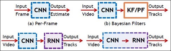
In this chapter, we will focus on the difference between CNN and RNN −
CNN
RNN
It is suitable for spatial data such as images.
RNN is suitable for temporal data, also called sequential data.
CNN is considered to be more powerful than RNN.
RNN includes less feature compatibility when compared to CNN.
This network takes fixed size inputs and generates fixed size outputs.
RNN can handle arbitrary input/output lengths.
CNN is a type of feed-forward artificial neural network with variations of multilayer perceptrons designed to use minimal amounts of preprocessing.
RNN unlike feed forward neural networks – can use their internal memory to process arbitrary sequences of inputs.
CNNs use connectivity pattern between the neurons. This is inspired by the organization of the animal visual cortex, whose individual neurons are arranged in such a way that they respond to overlapping regions tiling the visual field.
Recurrent neural networks use time-series information – what a user spoke last will impact what he/she will speak next.
CNNs are ideal for images and video processing.
RNNs are ideal for text and speech analysis.
Following illustration shows the schematic representation of CNN and RNN −
TFLearn can be defined as a modular and transparent deep learning aspect used in TensorFlow framework. The main motive of TFLearn is to provide a higher level API to TensorFlow for facilitating and showing up new experiments.
Consider the following important features of TFLearn −
TFLearn is easy to use and understand.
It includes easy concepts to build highly modular network layers, optimizers and various metrics embedded within them.
It includes full transparency with TensorFlow work system.
It includes powerful helper functions to train the built in tensors which accept multiple inputs, outputs and optimizers.
It includes easy and beautiful graph visualization.
The graph visualization includes various details of weights, gradients and activations.
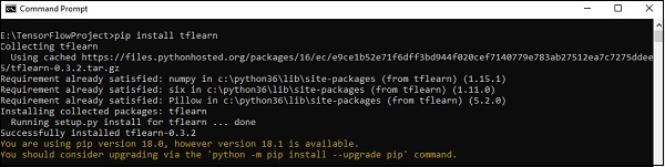
Install TFLearn by executing the following command −
pip install tflearn
Upon execution of the above code, the following output will be generated −
The following illustration shows the implementation of TFLearn with Random Forest classifier −
from __future__ import division, print_function, absolute_import

#TFLearn module implementation
import tflearn
from tflearn.estimators import RandomForestClassifier

# Data loading and pre-processing with respect to dataset
import tflearn.datasets.mnist as mnist
X, Y, testX, testY = mnist.load_data(one_hot = False)

m = RandomForestClassifier(n_estimators = 100, max_nodes = 1000)
m.fit(X, Y, batch_size = 10000, display_step = 10)

print("Compute the accuracy on train data:")
print(m.evaluate(X, Y, tflearn.accuracy_op))

print("Compute the accuracy on test set:")
print(m.evaluate(testX, testY, tflearn.accuracy_op))

print("Digits for test images id 0 to 5:")
print(m.predict(testX[:5]))

print("True digits:")
print(testY[:5])
In this chapter, we will focus on the basic example of linear regression implementation using TensorFlow. Logistic regression or linear regression is a supervised machine learning approach for the classification of order discrete categories. Our goal in this chapter is to build a model by which a user can predict the relationship between predictor variables and one or more independent variables.
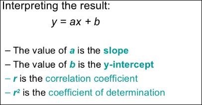
The relationship between these two variables is cons −idered linear. If y is the dependent variable and x is considered as the independent variable, then the linear regression relationship of two variables will look like the following equation −
Y = Ax+b
We will design an algorithm for linear regression. This will allow us to understand the following two important concepts −
Cost Function
Gradient descent algorithms
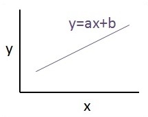
The schematic representation of linear regression is mentioned below −
The graphical view of the equation of linear regression is mentioned below −
Steps to design an algorithm for linear regression
We will now learn about the steps that help in designing an algorithm for linear regression.
Step 1
It is important to import the necessary modules for plotting the linear regression module. We start importing the Python library NumPy and Matplotlib.
import numpy as np
import matplotlib.pyplot as plt
Step 2
Define the number of coefficients necessary for logistic regression.
number_of_points = 500
x_point = []
y_point = []
a = 0.22
b = 0.78
Step 3
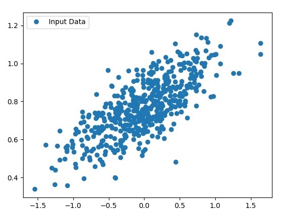
Iterate the variables for generating 300 random points around the regression equation −
Y = 0.22x+0.78
for i in range(number_of_points):
   x = np.random.normal(0.0,0.5)
   y = a*x + b +np.random.normal(0.0,0.1) x_point.append([x])
   y_point.append([y])
The complete code for logistic regression is as follows −
import numpy as np
import matplotlib.pyplot as plt

number_of_points = 500
x_point = []
y_point = []
a = 0.22
b = 0.78

for i in range(number_of_points):
   x = np.random.normal(0.0,0.5)
   y = a*x + b +np.random.normal(0.0,0.1) x_point.append([x])
   y_point.append([y])

plt.plot(x_point,y_point, 'o', label = 'Input Data') plt.legend()
plt.show()
The number of points which is taken as input is considered as input data.
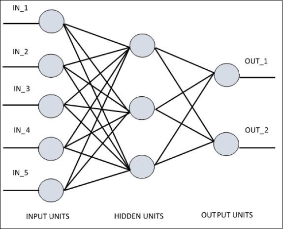
For understanding single layer perceptron, it is important to understand Artificial Neural Networks (ANN). Artificial neural networks is the information processing system the mechanism of which is inspired with the functionality of biological neural circuits. An artificial neural network possesses many processing units connected to each other. Following is the schematic representation of artificial neural network −
The diagram shows that the hidden units communicate with the external layer. While the input and output units communicate only through the hidden layer of the network.
The pattern of connection with nodes, the total number of layers and level of nodes between inputs and outputs with the number of neurons per layer define the architecture of a neural network.
There are two types of architecture. These types focus on the functionality artificial neural networks as follows −
Single Layer Perceptron
Multi-Layer Perceptron
Single Layer Perceptron
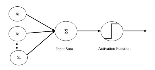
Single layer perceptron is the first proposed neural model created. The content of the local memory of the neuron consists of a vector of weights. The computation of a single layer perceptron is performed over the calculation of sum of the input vector each with the value multiplied by corresponding element of vector of the weights. The value which is displayed in the output will be the input of an activation function.
Let us focus on the implementation of single layer perceptron for an image classification problem using TensorFlow. The best example to illustrate the single layer perceptron is through representation of “Logistic Regression”.
Now, let us consider the following basic steps of training logistic regression −
The weights are initialized with random values at the beginning of the training.
For each element of the training set, the error is calculated with the difference between desired output and the actual output. The error calculated is used to adjust the weights.
The process is repeated until the error made on the entire training set is not less than the specified threshold, until the maximum number of iterations is reached.
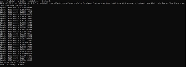
The complete code for evaluation of logistic regression is mentioned below −
# Import MINST data
from tensorflow.examples.tutorials.mnist import input_data
mnist = input_data.read_data_sets("/tmp/data/", one_hot = True)
import tensorflow as tf
import matplotlib.pyplot as plt
# Parameters
learning_rate = 0.01
training_epochs = 25
batch_size = 100
display_step = 1
# tf Graph Input
x = tf.placeholder("float", [None, 784]) # mnist data image of shape 28*28 = 784
y = tf.placeholder("float", [None, 10]) # 0-9 digits recognition => 10 classes
# Create model
# Set model weights
W = tf.Variable(tf.zeros([784, 10]))
b = tf.Variable(tf.zeros([10]))
# Construct model
activation = tf.nn.softmax(tf.matmul(x, W) + b) # Softmax
# Minimize error using cross entropy
cross_entropy = y*tf.log(activation)
cost = tf.reduce_mean\ (-tf.reduce_sum\ (cross_entropy,reduction_indices = 1))
optimizer = tf.train.\ GradientDescentOptimizer(learning_rate).minimize(cost)
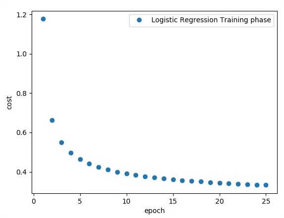
#Plot settings
avg_set = []
epoch_set = []
# Initializing the variables init = tf.initialize_all_variables()
# Launch the graph
with tf.Session() as sess:
sess.run(init)
# Training cycle
for epoch in range(training_epochs):
avg_cost = 0.
total_batch = int(mnist.train.num_examples/batch_size)
# Loop over all batches
for i in range(total_batch):
batch_xs, batch_ys = \ mnist.train.next_batch(batch_size)
# Fit training using batch data sess.run(optimizer, \ feed_dict = {
x: batch_xs, y: batch_ys})
# Compute average loss avg_cost += sess.run(cost, \ feed_dict = {
x: batch_xs, \ y: batch_ys})/total_batch
# Display logs per epoch step
if epoch % display_step == 0:
print ("Epoch:", '%04d' % (epoch+1), "cost=", "{:.9f}".format(avg_cost))
avg_set.append(avg_cost) epoch_set.append(epoch+1)
The logistic regression is considered as a predictive analysis. Logistic regression is used to describe data and to explain the relationship between one dependent binary variable and one or more nominal or independent variables.
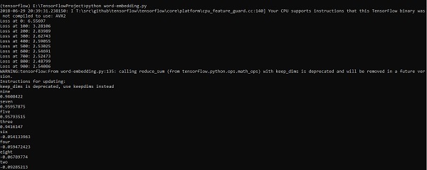
Word embedding is the concept of mapping from discrete objects such as words to vectors and real numbers. It is important for input for machine learning. The concept includes standard functions, which effectively transform discrete input objects to useful vectors.
The sample illustration of input of word embedding is as shown below −
Word2vec is the most common approach used for unsupervised word embedding technique. It trains the model in such a way that a given input word predicts the word’s context by using skip-grams.
TensorFlow enables many ways to implement this kind of model with increasing levels of sophistication and optimization and using multithreading concepts and higher-level abstractions.
import os
import math
import numpy as np
import tensorflow as tf
from tensorflow.contrib.tensorboard.plugins import projector
batch_size = 64
embedding_dimension = 5
negative_samples = 8
LOG_DIR = "logs/word2vec_intro"
digit_to_word_map = {
1: "One",
2: "Two",
3: "Three",
4: "Four",
5: "Five",
6: "Six",
7: "Seven",
8: "Eight",
9: "Nine"}
sentences = []
# Create two kinds of sentences - sequences of odd and even digits.
for i in range(10000):
rand_odd_ints = np.random.choice(range(1, 10, 2), 3)
sentences.append(" ".join([digit_to_word_map[r] for r in rand_odd_ints]))
sentences.append(" ".join([digit_to_word_map[r] for r in rand_even_ints]))
# Map words to indices
word2index_map = {}
index = 0
for sent in sentences:
for word in sent.lower().split():
if word not in word2index_map:
word2index_map[word] = index
index += 1
index2word_map = {index: word for word, index in word2index_map.items()}
vocabulary_size = len(index2word_map)
# Generate skip-gram pairs
skip_gram_pairs = []
for sent in sentences:
tokenized_sent = sent.lower().split()
for i in range(1, len(tokenized_sent)-1):
batch = instance_indices[:batch_size]
x = [skip_gram_pairs[i][0] for i in batch]
y = [[skip_gram_pairs[i][1]] for i in batch]
return x, y
# batch example
x_batch, y_batch = get_skipgram_batch(8)
x_batch
y_batch
[index2word_map[word] for word in x_batch] [index2word_map[word[0]] for word in y_batch]
# Input data, labels train_inputs = tf.placeholder(tf.int32, shape = [batch_size])
train_labels = tf.placeholder(tf.int32, shape = [batch_size, 1])
# Embedding lookup table currently only implemented in CPU with
tf.name_scope("embeddings"):
embeddings = tf.Variable(
tf.random_uniform([vocabulary_size, embedding_dimension], -1.0, 1.0),
name = 'embedding')
# This is essentialy a lookup table
embed = tf.nn.embedding_lookup(embeddings, train_inputs)
# Create variables for the NCE loss
nce_weights = tf.Variable(
tf.truncated_normal([vocabulary_size, embedding_dimension], stddev = 1.0 /
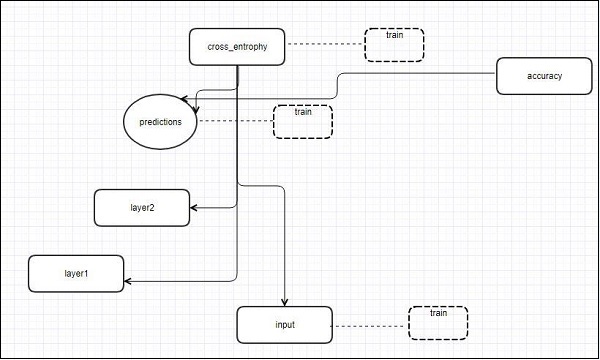
TensorFlow includes a visualization tool, which is called the TensorBoard. It is used for analyzing Data Flow Graph and also used to understand machine-learning models. The important feature of TensorBoard includes a view of different types of statistics about the parameters and details of any graph in vertical alignment.
Deep neural network includes up to 36,000 nodes. TensorBoard helps in collapsing these nodes in high-level blocks and highlighting the identical structures. This allows better analysis of graph focusing on the primary sections of the computation graph. The TensorBoard visualization is said to be very interactive where a user can pan, zoom and expand the nodes to display the details.
The following schematic diagram representation shows the complete working of TensorBoard visualization −
The algorithms collapse nodes into high-level blocks and highlight the specific groups with identical structures, which separate high-degree nodes. The TensorBoard thus created is useful and is treated equally important for tuning a machine learning model. This visualization tool is designed for the configuration log file with summary information and details that need to be displayed.
Let us focus on the demo example of TensorBoard visualization with the help of the following code −
import tensorflow as tf

# Constants creation for TensorBoard visualization
a = tf.constant(10,name = "a")
b = tf.constant(90,name = "b")
y = tf.Variable(a+b*2,name = 'y')
model = tf.initialize_all_variables() #Creation of model

with tf.Session() as session:
   merged = tf.merge_all_summaries()
   writer = tf.train.SummaryWriter("/tmp/tensorflowlogs",session.graph)
   session.run(model)
   print(session.run(y))
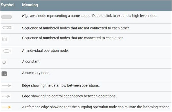
The following table shows the various symbols of TensorBoard visualization used for the node representation −
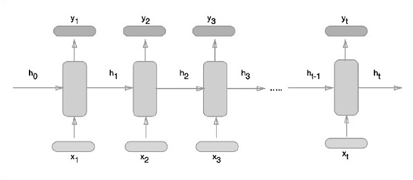
Recurrent neural networks is a type of deep learning-oriented algorithm, which follows a sequential approach. In neural networks, we always assume that each input and output is independent of all other layers. These type of neural networks are called recurrent because they perform mathematical computations in sequential manner.
Consider the following steps to train a recurrent neural network −
Step 1 − Input a specific example from dataset.
Step 2 − Network will take an example and compute some calculations using randomly initialized variables.
Step 3 − A predicted result is then computed.
Step 4 − The comparison of actual result generated with the expected value will produce an error.
Step 5 − To trace the error, it is propagated through same path where the variables are also adjusted.
Step 6 − The steps from 1 to 5 are repeated until we are confident that the variables declared to get the output are defined properly.
Step 7 − A systematic prediction is made by applying these variables to get new unseen input.
The schematic approach of representing recurrent neural networks is described below −
Recurrent Neural Network Implementation with TensorFlow
In this section, we will learn how to implement recurrent neural network with TensorFlow.
Step 1 − TensorFlow includes various libraries for specific implementation of the recurrent neural network module.
#Import necessary modules
from __future__ import print_function

import tensorflow as tf
from tensorflow.contrib import rnn
from tensorflow.examples.tutorials.mnist import input_data
mnist = input_data.read_data_sets("/tmp/data/", one_hot = True)
As mentioned above, the libraries help in defining the input data, which forms the primary part of recurrent neural network implementation.
Step 2 − Our primary motive is to classify the images using a recurrent neural network, where we consider every image row as a sequence of pixels. MNIST image shape is specifically defined as 28*28 px. Now we will handle 28 sequences of 28 steps for each sample that is mentioned. We will define the input parameters to get the sequential pattern done.
Step 3 − Compute the results using a defined function in RNN to get the best results. Here, each data shape is compared with current input shape and the results are computed to maintain the accuracy rate.
def RNN(x, weights, biases):
   x = tf.unstack(x, n_steps, 1)

   # Define a lstm cell with tensorflow
   lstm_cell = rnn.BasicLSTMCell(n_hidden, forget_bias=1.0)

   # Get lstm cell output
   outputs, states = rnn.static_rnn(lstm_cell, x, dtype = tf.float32)

   # Linear activation, using rnn inner loop last output
   return tf.matmul(outputs[-1], weights['out']) + biases['out']

pred = RNN(x, weights, biases)

# Define loss and optimizer
cost = tf.reduce_mean(tf.nn.softmax_cross_entropy_with_logits(logits = pred, labels = y))
optimizer = tf.train.AdamOptimizer(learning_rate = learning_rate).minimize(cost)

# Evaluate model
correct_pred = tf.equal(tf.argmax(pred,1), tf.argmax(y,1))
accuracy = tf.reduce_mean(tf.cast(correct_pred, tf.float32))

# Initializing the variables
init = tf.global_variables_initializer()
Step 4 − In this step, we will launch the graph to get the computational results. This also helps in calculating the accuracy for test results.
with tf.Session() as sess:
sess.run(init)
step = 1
# Keep training until reach max iterations
while step * batch_size < training_iters:
After understanding machine-learning concepts, we can now shift our focus to deep learning concepts. Deep learning is a division of machine learning and is considered as a crucial step taken by researchers in recent decades. The examples of deep learning implementation include applications like image recognition and speech recognition.
Following are the two important types of deep neural networks −
Convolutional Neural Networks
Recurrent Neural Networks
In this chapter, we will focus on the CNN, Convolutional Neural Networks.
Convolutional Neural Networks
Convolutional Neural networks are designed to process data through multiple layers of arrays. This type of neural networks is used in applications like image recognition or face recognition. The primary difference between CNN and any other ordinary neural network is that CNN takes input as a two-dimensional array and operates directly on the images rather than focusing on feature extraction which other neural networks focus on.
The dominant approach of CNN includes solutions for problems of recognition. Top companies like Google and Facebook have invested in research and development towards recognition projects to get activities done with greater speed.
A convolutional neural network uses three basic ideas −
Local respective fields
Convolution
Pooling
Let us understand these ideas in detail.
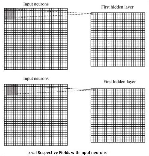
CNN utilizes spatial correlations that exist within the input data. Each concurrent layer of a neural network connects some input neurons. This specific region is called local receptive field. Local receptive field focusses on the hidden neurons. The hidden neurons process the input data inside the mentioned field not realizing the changes outside the specific boundary.
Following is a diagram representation of generating local respective fields −
If we observe the above representation, each connection learns a weight of the hidden neuron with an associated connection with movement from one layer to another. Here, individual neurons perform a shift from time to time. This process is called “convolution”.
The mapping of connections from the input layer to the hidden feature map is defined as “shared weights” and bias included is called “shared bias”.
CNN or convolutional neural networks use pooling layers, which are the layers, positioned immediately after CNN declaration. It takes the input from the user as a feature map that comes out of convolutional networks and prepares a condensed feature map. Pooling layers helps in creating layers with neurons of previous layers.
TensorFlow Implementation of CNN
In this section, we will learn about the TensorFlow implementation of CNN. The steps,which require the execution and proper dimension of the entire network, are as shown below −
Step 1 − Include the necessary modules for TensorFlow and the data set modules, which are needed to compute the CNN model.
import tensorflow as tf
import numpy as np
from tensorflow.examples.tutorials.mnist import input_data
Step 2 − Declare a function called run_cnn(), which includes various parameters and optimization variables with declaration of data placeholders. These optimization variables will declare the training pattern.
Step 3 − In this step, we will declare the training data placeholders with input parameters – for 28 x 28 pixels = 784. This is the flattened image data that is drawn from mnist.train.nextbatch().
We can reshape the tensor according to our requirements. The first value (-1) tells function to dynamically shape that dimension based on the amount of data passed to it. The two middle dimensions are set to the image size (i.e. 28 x 28).
x = tf.placeholder(tf.float32, [None, 784])
x_shaped = tf.reshape(x, [-1, 28, 28, 1])
y = tf.placeholder(tf.float32, [None, 10])
Step 4 − Now it is important to create some convolutional layers −
Step 5 − Let us flatten the output ready for the fully connected output stage – after two layers of stride 2 pooling with the dimensions of 28 x 28, to dimension of 14 x 14 or minimum 7 x 7 x,y co-ordinates, but with 64 output channels. To create the fully connected with “dense” layer, the new shape needs to be [-1, 7 x 7 x 64]. We can set up some weights and bias values for this layer, then activate with ReLU.
Step 6 − Another layer with specific softmax activations with the required optimizer defines the accuracy assessment, which makes the setup of initialization operator.
return out_layer
if __name__ == "__main__":
run_cnn()
Following is the output generated by the above code −
See @{tf.nn.softmax_cross_entropy_with_logits_v2}.
2018-09-19 17:22:58.802268: I
T:\src\github\tensorflow\tensorflow\core\platform\cpu_feature_guard.cc:140]
Your CPU supports instructions that this TensorFlow binary was not compiled to
use: AVX2
2018-09-19 17:25:41.522845: W
T:\src\github\tensorflow\tensorflow\core\framework\allocator.cc:101] Allocation
of 1003520000 exceeds 10% of system memory.
2018-09-19 17:25:44.630941: W
T:\src\github\tensorflow\tensorflow\core\framework\allocator.cc:101] Allocation
of 501760000 exceeds 10% of system memory.
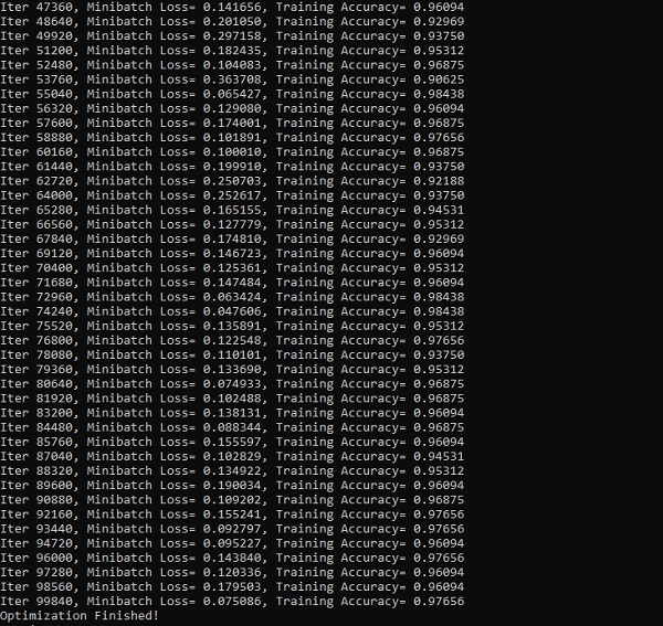
Epoch: 1 cost = 0.676 test accuracy: 0.940
2018-09-19 17:26:51.987554: W
T:\src\github\tensorflow\tensorflow\core\framework\allocator.cc:101] Allocation
of 1003520000 exceeds 10% of system memory.
In this chapter, we will learn about the basics of TensorFlow. We will begin by understanding the data structure of tensor.
Tensor Data Structure
Tensors are used as the basic data structures in TensorFlow language. Tensors represent the connecting edges in any flow diagram called the Data Flow Graph. Tensors are defined as multidimensional array or list.
Tensors are identified by the following three parameters −
Rank
Unit of dimensionality described within tensor is called rank. It identifies the number of dimensions of the tensor. A rank of a tensor can be described as the order or n-dimensions of a tensor defined.
Shape
The number of rows and columns together define the shape of Tensor.
Type
Type describes the data type assigned to Tensor’s elements.
A user needs to consider the following activities for building a Tensor −
Build an n-dimensional array
Convert the n-dimensional array.
Various Dimensions of TensorFlow
TensorFlow includes various dimensions. The dimensions are described in brief below −
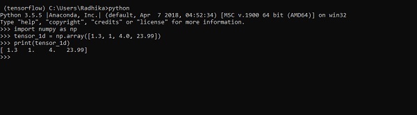
One dimensional Tensor
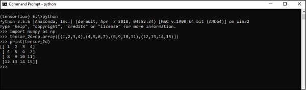
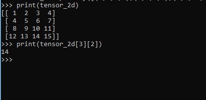
One dimensional tensor is a normal array structure which includes one set of values of the same data type.
The implementation with the output is shown in the screenshot below −
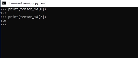
The indexing of elements is same as Python lists. The first element starts with index of 0; to print the values through index, all you need to do is mention the index number.
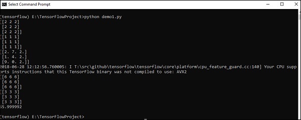
The above code will generate the following output −
Explanation
We have created multidimensional arrays in the above source code. Now, it is important to understand that we created graph and sessions, which manage the Tensors and generate the appropriate output. With the help of graph, we have the output specifying the mathematical calculations between Tensors.