In this chapter, we will understand the various aspects of neural network training which can be implemented using TensorFlow framework.
Following are the ten recommendations, which can be evaluated −
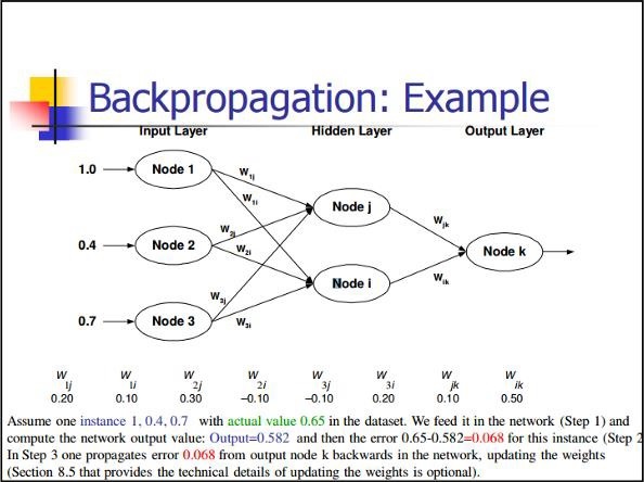
Back Propagation
Back propagation is a simple method to compute partial derivatives, which includes the basic form of composition best suitable for neural nets.
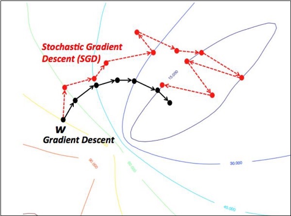
Stochastic Gradient Descent
In stochastic gradient descent, a batch is the total number of examples, which a user uses to calculate the gradient in a single iteration. So far, it is assumed that the batch has been the entire data set. The best illustration is working at Google scale; data sets often contain billions or even hundreds of billions of examples.
Explore our latest online courses and learn new skills at your own pace. Enroll and become a certified expert to boost your career.
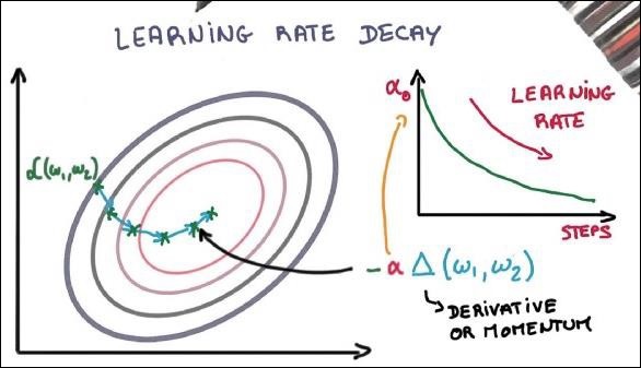
Learning Rate Decay
Adapting the learning rate is one of the most important features of gradient descent optimization. This is crucial to TensorFlow implementation.
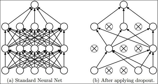
Dropout
Deep neural nets with a large number of parameters form powerful machine learning systems. However, over fitting is a serious problem in such networks.
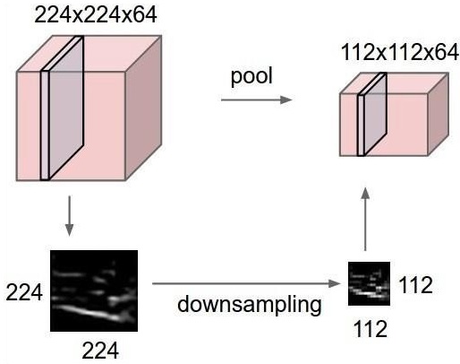
Max Pooling
Max pooling is a sample-based discretization process. The object is to down-sample an input representation, which reduces the dimensionality with the required assumptions.
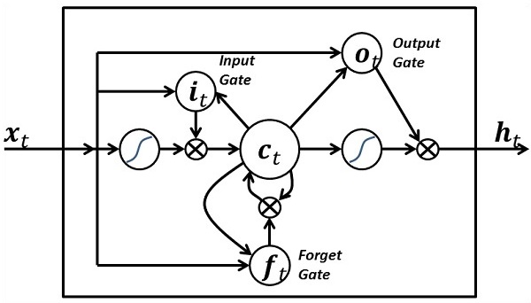
Long Short Term Memory (LSTM)
LSTM controls the decision on what inputs should be taken within the specified neuron. It includes the control on deciding what should be computed and what output should be generated.
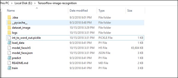
TensorFlow includes a special feature of image recognition and these images are stored in a specific folder. With relatively same images, it will be easy to implement this logic for security purposes.
The folder structure of image recognition code implementation is as shown below −
The dataset_image includes the related images, which need to be loaded. We will focus on image recognition with our logo defined in it. The images are loaded with “load_data.py” script, which helps in keeping a note on various image recognition modules within them.
import pickle
from sklearn.model_selection import train_test_split
from scipy import misc
import numpy as np
import os
label = os.listdir("dataset_image")
label = label[1:]
dataset = []
for image_label in label:
images = os.listdir("dataset_image/"+image_label)
for image in images:
X = []
Y = []
for input,image_label in dataset:
X.append(input)
Y.append(label.index(image_label))
X = np.array(X)
Y = np.array(Y)
X_train,y_train, = X,Y
data_set = (X_train,y_train)
save_label = open("int_to_word_out.pickle","wb")
pickle.dump(label, save_label)
save_label.close()
The training of images helps in storing the recognizable patterns within specified folder.
import numpy
import matplotlib.pyplot as plt
from keras.layers import Dropout
from keras.layers import Flatten
from keras.constraints import maxnorm
from keras.optimizers import SGD
from keras.layers import Conv2D
from keras.layers.convolutional import MaxPooling2D
from keras.utils import np_utils
from keras import backend as K
import load_data
from keras.models import Sequential
from keras.layers import Dense
import keras
K.set_image_dim_ordering('tf')
# fix random seed for reproducibility
seed = 7
numpy.random.seed(seed)
# load data
(X_train,y_train) = load_data.data_set
# normalize inputs from 0-255 to 0.0-1.0
X_train = X_train.astype('float32')
#X_test = X_test.astype('float32')
X_train = X_train / 255.0
#X_test = X_test / 255.0
# one hot encode outputs
y_train = np_utils.to_categorical(y_train)
#y_test = np_utils.to_categorical(y_test)
num_classes = y_train.shape[1]
# Create the model
model = Sequential()
model.add(Conv2D(32, (3, 3), input_shape = (64, 64, 3), padding = 'same',
activation = 'relu', kernel_constraint = maxnorm(3)))
model.add(Dropout(0.2))
model.add(Conv2D(32, (3, 3), activation = 'relu', padding = 'same',
kernel_constraint = maxnorm(3)))
model.add(MaxPooling2D(pool_size = (2, 2)))
model.add(Flatten())
model.add(Dense(512, activation = 'relu', kernel_constraint = maxnorm(3)))
model.add(Dropout(0.5))
model.add(Dense(num_classes, activation = 'softmax'))
# Compile model
epochs = 10
lrate = 0.01
decay = lrate/epochs
sgd = SGD(lr = lrate, momentum = 0.9, decay = decay, nesterov = False)
model.compile(loss = 'categorical_crossentropy', optimizer = sgd, metrics = ['accuracy'])
print(model.summary())
#callbacks = [keras.callbacks.EarlyStopping(
monitor = 'val_loss', min_delta = 0, patience = 0, verbose = 0, mode = 'auto')]
callbacks = [keras.callbacks.TensorBoard(log_dir='./logs',
histogram_freq = 0, batch_size = 32, write_graph = True, write_grads = False,
write_images = True, embeddings_freq = 0, embeddings_layer_names = None,
embeddings_metadata = None)]
# Fit the model
model.fit(X_train, y_train, epochs = epochs,
batch_size = 32,shuffle = True,callbacks = callbacks)
# Final evaluation of the model
scores = model.evaluate(X_train, y_train, verbose = 0)
print("Accuracy: %.2f%%" % (scores[1]*100))
# serialize model to JSONx
model_json = model.to_json()
with open("model_face.json", "w") as json_file:
json_file.write(model_json)
# serialize weights to HDF5
model.save_weights("model_face.h5")
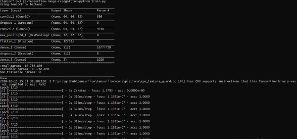
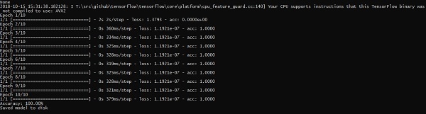
print("Saved model to disk")
The above line of code generates an output as shown below −
A partial differential equation (PDE) is a differential equation, which involves partial derivatives with unknown function of several independent variables. With reference to partial differential equations, we will focus on creating new graphs.
Let us assume there is a pond with dimension 500*500 square −
N = 500
Now, we will compute partial differential equation and form the respective graph using it. Consider the steps given below for computing graph.
Step 1 − Import libraries for simulation.
import tensorflow as tf
import numpy as np
import matplotlib.pyplot as plt
Step 2 − Include functions for transformation of a 2D array into a convolution kernel and simplified 2D convolution operation.
def make_kernel(a):
   a = np.asarray(a)
   a = a.reshape(list(a.shape) + [1,1])
   return tf.constant(a, dtype=1)

def simple_conv(x, k):
   """A simplified 2D convolution operation"""
   x = tf.expand_dims(tf.expand_dims(x, 0), -1)
   y = tf.nn.depthwise_conv2d(x, k, [1, 1, 1, 1], padding = 'SAME')
   return y[0, :, :, 0]

def laplace(x):
   """Compute the 2D laplacian of an array"""
   laplace_k = make_kernel([[0.5, 1.0, 0.5], [1.0, -6., 1.0], [0.5, 1.0, 0.5]])
   return simple_conv(x, laplace_k)

sess = tf.InteractiveSession()
Step 3 − Include the number of iterations and compute the graph to display the records accordingly.
N = 500
# Initial Conditions -- some rain drops hit a pond
# Set everything to zero
u_init = np.zeros([N, N], dtype = np.float32)
ut_init = np.zeros([N, N], dtype = np.float32)
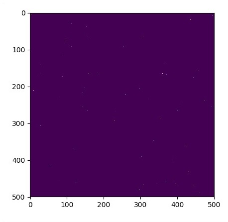
# Some rain drops hit a pond at random points
for n in range(100):
a,b = np.random.randint(0, N, 2)
u_init[a,b] = np.random.uniform()
plt.imshow(u_init)
plt.show()
# Parameters:
# eps -- time resolution
# damping -- wave damping
eps = tf.placeholder(tf.float32, shape = ())
damping = tf.placeholder(tf.float32, shape = ())
# Create variables for simulation state
U = tf.Variable(u_init)
Ut = tf.Variable(ut_init)
# Discretized PDE update rules
U_ = U + eps * Ut
Ut_ = Ut + eps * (laplace(U) - damping * Ut)
# Operation to update the state
step = tf.group(U.assign(U_), Ut.assign(Ut_))
# Initialize state to initial conditions
tf.initialize_all_variables().run()
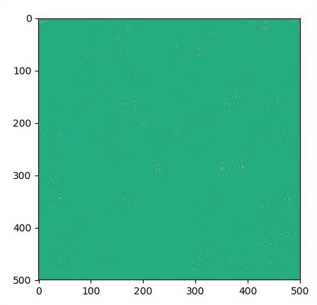
# Run 1000 steps of PDE
for i in range(1000):
# Step simulation
step.run({eps: 0.03, damping: 0.04})
# Visualize every 50 steps
if i % 500 == 0:
In this chapter, we will learn about the XOR implementation using TensorFlow. Before starting with XOR implementation in TensorFlow, let us see the XOR table values. This will help us understand encryption and decryption process.
A
B
A XOR B
0
0
0
0
1
1
1
0
1
1
1
0
XOR Cipher encryption method is basically used to encrypt data which is hard to crack with brute force method, i.e., by generating random encryption keys which match the appropriate key.
The concept of implementation with XOR Cipher is to define a XOR encryption key and then perform XOR operation of the characters in the specified string with this key, which a user tries to encrypt. Now we will focus on XOR implementation using TensorFlow, which is mentioned below −
#Declaring necessary modules
import tensorflow as tf
import numpy as np
"""
A simple numpy implementation of a XOR gate to understand the backpropagation
algorithm
"""
x = tf.placeholder(tf.float64,shape = [4,2],name = "x")
#declaring a place holder for input x
y = tf.placeholder(tf.float64,shape = [4,1],name = "y")
#declaring a place holder for desired output y
m = np.shape(x)[0]#number of training examples
n = np.shape(x)[1]#number of features
hidden_s = 2 #number of nodes in the hidden layer
l_r = 1#learning rate initialization
theta1 = tf.cast(tf.Variable(tf.random_normal([3,hidden_s]),name = "theta1"),tf.float64)
theta2 = tf.cast(tf.Variable(tf.random_normal([hidden_s+1,1]),name = "theta2"),tf.float64)
#conducting forward propagation
a1 = tf.concat([np.c_[np.ones(x.shape[0])],x],1)
#the weights of the first layer are multiplied by the input of the first layer
z1 = tf.matmul(a1,theta1)
#the input of the second layer is the output of the first layer, passed through the
activation function and column of biases is added
a2 = tf.concat([np.c_[np.ones(x.shape[0])],tf.sigmoid(z1)],1)
#the input of the second layer is multiplied by the weights
z3 = tf.matmul(a2,theta2)
#the output is passed through the activation function to obtain the final probability
h3 = tf.sigmoid(z3)
cost_func = -tf.reduce_sum(y*tf.log(h3)+(1-y)*tf.log(1-h3),axis = 1)
#built in tensorflow optimizer that conducts gradient descent using specified
learning rate to obtain theta values
optimiser = tf.train.GradientDescentOptimizer(learning_rate = l_r).minimize(cost_func)
#setting required X and Y values to perform XOR operation
X = [[0,0],[0,1],[1,0],[1,1]]
Y = [[0],[1],[1],[0]]
#initializing all variables, creating a session and running a tensorflow session
init = tf.global_variables_initializer()
sess = tf.Session()
sess.run(init)
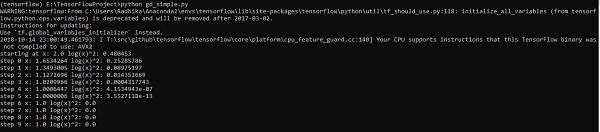
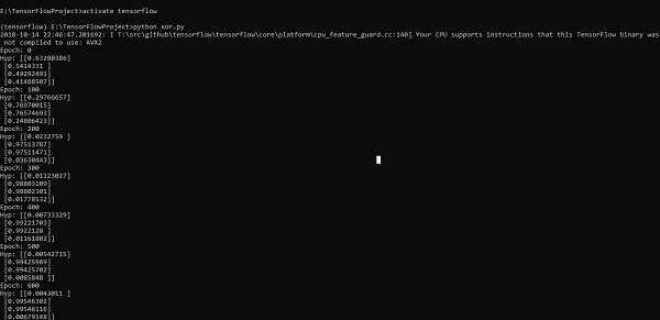
#running gradient descent for each iteration and printing the hypothesis
obtained using the updated theta values
for i in range(100000):
sess.run(optimiser, feed_dict = {x:X,y:Y})#setting place holder values using feed_dict
if i%100==0:
Optimizers are the extended class, which include added information to train a specific model. The optimizer class is initialized with given parameters but it is important to remember that no Tensor is needed. The optimizers are used for improving speed and performance for training a specific model.
The basic optimizer of TensorFlow is −
tf.train.Optimizer
This class is defined in the specified path of tensorflow/python/training/optimizer.py.
Following are some optimizers in Tensorflow −
Stochastic Gradient descent
Stochastic Gradient descent with gradient clipping
Momentum
Nesterov momentum
Adagrad
Adadelta
RMSProp
Adam
Adamax
SMORMS3
We will focus on the Stochastic Gradient descent. The illustration for creating optimizer for the same is mentioned below −
def sgd(cost, params, lr = np.float32(0.01)):
   g_params = tf.gradients(cost, params)
   updates = []

   for param, g_param in zip(params, g_params):
  updates.append(param.assign(param - lr*g_param))   return updates
The basic parameters are defined within the specific function. In our subsequent chapter, we will focus on Gradient Descent Optimization with implementation of optimizers.
In this chapter, we will be focus on the network we will have to learn from known set of points called x and f(x). A single hidden layer will build this simple network.
The code for the explanation of hidden layers of perceptron is as shown below −
#Importing the necessary modules
import tensorflow as tf
import numpy as np
import math, random
import matplotlib.pyplot as plt
np.random.seed(1000)
function_to_learn = lambda x: np.cos(x) + 0.1*np.random.randn(*x.shape)
layer_1_neurons = 10
NUM_points = 1000
#Training the parameters
batch_size = 100
NUM_EPOCHS = 1500
all_x = np.float32(np.random.uniform(-2*math.pi, 2*math.pi, (1, NUM_points))).T
np.random.shuffle(all_x)
train_size = int(900)
#Training the first 700 points in the given set x_training = all_x[:train_size]
y_training = function_to_learn(x_training)
#Training the last 300 points in the given set x_validation = all_x[train_size:]
y_validation = function_to_learn(x_validation)
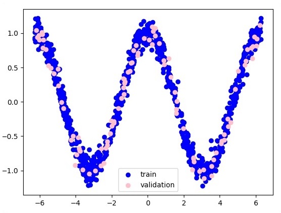
plt.figure(1)
plt.scatter(x_training, y_training, c = 'blue', label = 'train')
plt.scatter(x_validation, y_validation, c = 'pink', label = 'validation')
plt.legend()
plt.show()
X = tf.placeholder(tf.float32, [None, 1], name = "X")
Y = tf.placeholder(tf.float32, [None, 1], name = "Y")
#first layer
#Number of neurons = 10
w_h = tf.Variable(
tf.random_uniform([1, layer_1_neurons],\ minval = -1, maxval = 1, dtype = tf.float32))
b_h = tf.Variable(tf.zeros([1, layer_1_neurons], dtype = tf.float32))
h = tf.nn.sigmoid(tf.matmul(X, w_h) + b_h)
#output layer
#Number of neurons = 10
w_o = tf.Variable(
tf.random_uniform([layer_1_neurons, 1],\ minval = -1, maxval = 1, dtype = tf.float32))
b_o = tf.Variable(tf.zeros([1, 1], dtype = tf.float32))
#build the model
model = tf.matmul(h, w_o) + b_o
#minimize the cost function (model - Y)
train_op = tf.train.AdamOptimizer().minimize(tf.nn.l2_loss(model - Y))
#Start the Learning phase
sess = tf.Session() sess.run(tf.initialize_all_variables())
errors = []
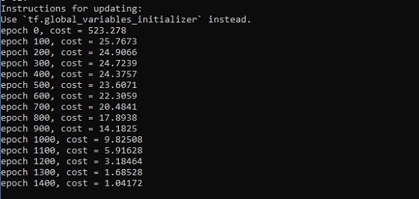
for i in range(NUM_EPOCHS):
for start, end in zip(range(0, len(x_training), batch_size),\
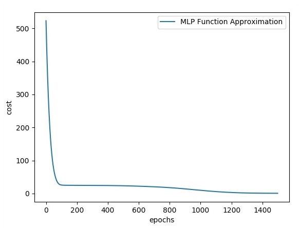
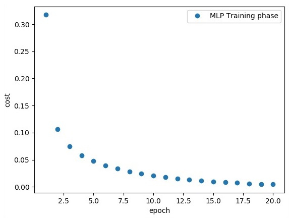
plt.plot(errors,label='MLP Function Approximation') plt.xlabel('epochs')
plt.ylabel('cost')
plt.legend()
plt.show()
Output
Following is the representation of function layer approximation −
Here two data are represented in shape of W. The two data are: train and validation which are represented in distinct colors as visible in legend section.
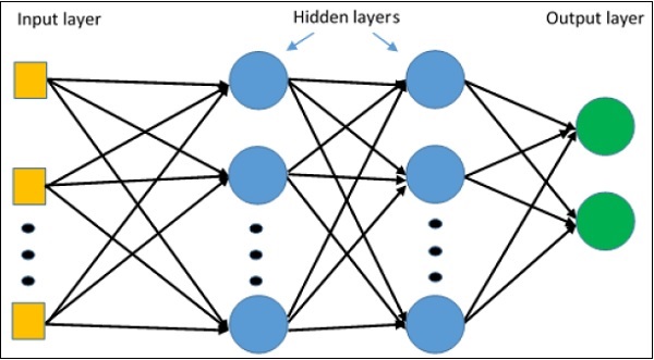
Multi-Layer perceptron defines the most complicated architecture of artificial neural networks. It is substantially formed from multiple layers of perceptron.
The diagrammatic representation of multi-layer perceptron learning is as shown below −
MLP networks are usually used for supervised learning format. A typical learning algorithm for MLP networks is also called back propagation’s algorithm.
Now, we will focus on the implementation with MLP for an image classification problem.
# Import MINST data
from tensorflow.examples.tutorials.mnist import input_data
mnist = input_data.read_data_sets("/tmp/data/", one_hot = True)
import tensorflow as tf
import matplotlib.pyplot as plt
# Parameters
learning_rate = 0.001
training_epochs = 20
batch_size = 100
display_step = 1
# Network Parameters
n_hidden_1 = 256
# 1st layer num features
n_hidden_2 = 256 # 2nd layer num features
n_input = 784 # MNIST data input (img shape: 28*28) n_classes = 10
# MNIST total classes (0-9 digits)
# tf Graph input
x = tf.placeholder("float", [None, n_input])
y = tf.placeholder("float", [None, n_classes])
# weights layer 1
h = tf.Variable(tf.random_normal([n_input, n_hidden_1])) # bias layer 1
bias_layer_1 = tf.Variable(tf.random_normal([n_hidden_1]))
# layer 1 layer_1 = tf.nn.sigmoid(tf.add(tf.matmul(x, h), bias_layer_1))
# weights layer 2
w = tf.Variable(tf.random_normal([n_hidden_1, n_hidden_2]))
# bias layer 2
bias_layer_2 = tf.Variable(tf.random_normal([n_hidden_2]))
# layer 2
layer_2 = tf.nn.sigmoid(tf.add(tf.matmul(layer_1, w), bias_layer_2))
# weights output layer
output = tf.Variable(tf.random_normal([n_hidden_2, n_classes]))
# biar output layer
bias_output = tf.Variable(tf.random_normal([n_classes])) # output layer
output_layer = tf.matmul(layer_2, output) + bias_output
# cost function
cost = tf.reduce_mean(tf.nn.sigmoid_cross_entropy_with_logits(
logits = output_layer, labels = y))
#cost = tf.reduce_mean(tf.nn.sigmoid_cross_entropy_with_logits(output_layer, y))
# optimizer
optimizer = tf.train.AdamOptimizer(learning_rate = learning_rate).minimize(cost)
# optimizer = tf.train.GradientDescentOptimizer(
learning_rate = learning_rate).minimize(cost)
# Plot settings
avg_set = []
epoch_set = []
# Initializing the variables
init = tf.global_variables_initializer()
# Launch the graph
with tf.Session() as sess:
sess.run(init)
# Training cycle
for epoch in range(training_epochs):
avg_cost = 0.
total_batch = int(mnist.train.num_examples / batch_size)
# Loop over all batches
for i in range(total_batch):
batch_xs, batch_ys = mnist.train.next_batch(batch_size)
# Fit training using batch data sess.run(optimizer, feed_dict = {
x: batch_xs, y: batch_ys})
# Compute average loss
avg_cost += sess.run(cost, feed_dict = {x: batch_xs, y: batch_ys}) / total_batch
# Display logs per epoch step
if epoch % display_step == 0:
print
Epoch:", '%04d' % (epoch + 1), "cost=", "{:.9f}".format(avg_cost)
avg_set.append(avg_cost)
epoch_set.append(epoch + 1)
Here, we will focus on MetaGraph formation in TensorFlow. This will help us understand export module in TensorFlow. The MetaGraph contains the basic information, which is required to train, perform evaluation, or run inference on a previously trained graph.
Following is the code snippet for the same −
def export_meta_graph(filename = None, collection_list = None, as_text = False):
   """this code writes MetaGraphDef to save_path/filename.

   Arguments:
   filename: Optional meta_graph filename including the path. collection_list:
  List of string keys to collect. as_text: If True,
  writes the meta_graph as an ASCII proto.
   Returns:
   A MetaGraphDef proto. """
One of the typical usage model for the same is mentioned below −
# Build the model ...
with tf.Session() as sess:
   # Use the model ...
# Export the model to /tmp/my-model.meta.
meta_graph_def = tf.train.export_meta_graph(filename = '/tmp/my-model.meta')
This chapter will focus on how to get started with distributed TensorFlow. The aim is to help developers understand the basic distributed TF concepts that are reoccurring, such as TF servers. We will use the Jupyter Notebook for evaluating distributed TensorFlow. The implementation of distributed computing with TensorFlow is mentioned below −
Step 1 − Import the necessary modules mandatory for distributed computing −
import tensorflow as tf
Step 2 − Create a TensorFlow cluster with one node. Let this node be responsible for a job that that has name “worker” and that will operate one take at localhost:2222.
cluster_spec = tf.train.ClusterSpec({'worker' : ['localhost:2222']})
server = tf.train.Server(cluster_spec)
server.target
The above scripts generate the following output −
'grpc://localhost:2222'
The server is currently running.
Step 3 − The server configuration with respective session can be calculated by executing the following command −
server.server_def
The above command generates the following output −
cluster {
   job {
  name: "worker"
  tasks {
     value: "localhost:2222"
  }   }
}
job_name: "worker"
protocol: "grpc"
Step 4 − Launch a TensorFlow session with the execution engine being the server. Use TensorFlow to create a local server and use lsof to find out the location of the server.
sess = tf.Session(target = server.target)
server = tf.train.Server.create_local_server()
Step 5 − View devices available in this session and close the respective session.
devices = sess.list_devices()
for d in devices:
   print(d.name)
sess.close()
The above command generates the following output −