alpha controls the width of the network. If the value is below 1, decreases the number of filters in each layer. If the value is above 1, increases the number of filters in each layer. If alpha = 1, default number of filters from the paper are used at each layer.
The default input size for this model is 224×224.
Explore our latest online courses and learn new skills at your own pace. Enroll and become a certified expert to boost your career.
InceptionResNetV2
InceptionResNetV2 is another pre-trained model. It is also trained using ImageNet. The syntax to load the model is as follows −
Keras is very simple, extensible and easy to implement neural network API, which can be used to build deep learning applications with high level abstraction. Keras is an optimal choice for deep leaning models.
include_top refers the fully-connected layer at the top of the network.
weights refer pre-training on ImageNet.
input_tensor refers optional Keras tensor to use as image input for the model.
input_shape refers optional shape tuple. The default input size for this model is 224×224.
classes refer optional number of classes to classify images.
Let us understand the model by writing a simple example −
Step 1: import the modules
Let us load the necessary modules as specified below −
>>> import PIL
>>> from keras.preprocessing.image import load_img
>>> from keras.preprocessing.image import img_to_array
>>> from keras.applications.imagenet_utils import decode_predictions
>>> import matplotlib.pyplot as plt
>>> import numpy as np
>>> from keras.applications.resnet50 import ResNet50
>>> from keras.applications import resnet50
Step 2: Select an input
Let us choose an input image, Lotus as specified below −
>>> filename = 'banana.jpg'
>>> ## load an image in PIL format
>>> original = load_img(filename, target_size = (224, 224))
>>> print('PIL image size',original.size)
PIL image size (224, 224)
>>> plt.imshow(original)
<matplotlib.image.AxesImage object at 0x1304756d8>
>>> plt.show()
Here, we have loaded an image (banana.jpg) and displayed it.
Explore our latest online courses and learn new skills at your own pace. Enroll and become a certified expert to boost your career.
Step 3: Convert images into NumPy array
Let us convert our input, Banana into NumPy array, so that it can be passed into the model for the purpose of prediction.
>>> #convert the PIL image to a numpy array
>>> numpy_image = img_to_array(original)

>>> plt.imshow(np.uint8(numpy_image))
<matplotlib.image.AxesImage object at 0x130475ac8>

>>> print('numpy array size',numpy_image.shape)
numpy array size (224, 224, 3)

>>> # Convert the image / images into batch format
>>> image_batch = np.expand_dims(numpy_image, axis = 0)

>>> print('image batch size', image_batch.shape)
image batch size (1, 224, 224, 3)
>>>
Step 4: Model prediction
Let us feed our input into the model to get the predictions
>>> prepare the image for the resnet50 model >>>
>>> processed_image = resnet50.preprocess_input(image_batch.copy())

>>> # create resnet model
>>>resnet_model = resnet50.ResNet50(weights = 'imagenet')
>>> Downloavding data from https://github.com/fchollet/deep-learning-models/releas
es/download/v0.2/resnet50_weights_tf_dim_ordering_tf_kernels.h5
102858752/102853048 [==============================] - 33s 0us/step

>>> # get the predicted probabilities for each class
>>> predictions = resnet_model.predict(processed_image)

>>> # convert the probabilities to class labels
>>> label = decode_predictions(predictions)
Downloading data from https://storage.googleapis.com/download.tensorflow.org/
data/imagenet_class_index.json
40960/35363 [==================================] - 0s 0us/step

>>> print(label)
Keras applications module is used to provide pre-trained model for deep neural networks. Keras models are used for prediction, feature extraction and fine tuning. This chapter explains about Keras applications in detail.
Pre-trained models
Trained model consists of two parts model Architecture and model Weights. Model weights are large file so we have to download and extract the feature from ImageNet database. Some of the popular pre-trained models are listed below,
ResNet
VGG16
MobileNet
InceptionResNetV2
InceptionV3
Loading a model
Keras pre-trained models can be easily loaded as specified below −
import keras
import numpy as np

from keras.applications import vgg16, inception_v3, resnet50, mobilenet

#Load the VGG model
vgg_model = vgg16.VGG16(weights = 'imagenet')

#Load the Inception_V3 model
inception_model = inception_v3.InceptionV3(weights = 'imagenet')

#Load the ResNet50 model
resnet_model = resnet50.ResNet50(weights = 'imagenet')

#Load the MobileNet model mobilenet_model = mobilenet.MobileNet(weights = 'imagenet')
Once the model is loaded, we can immediately use it for prediction purpose. Let us check each pre-trained model in the upcoming chapters.
In this chapter, let us write a simple Long Short Term Memory (LSTM) based RNN to do sequence analysis. A sequence is a set of values where each value corresponds to a particular instance of time. Let us consider a simple example of reading a sentence. Reading and understanding a sentence involves reading the word in the given order and trying to understand each word and its meaning in the given context and finally understanding the sentence in a positive or negative sentiment.
Here, the words are considered as values, and first value corresponds to first word, second value corresponds to second word, etc., and the order will be strictly maintained. Sequence Analysis is used frequently in natural language processing to find the sentiment analysis of the given text.
Let us create a LSTM model to analyze the IMDB movie reviews and find its positive/negative sentiment.
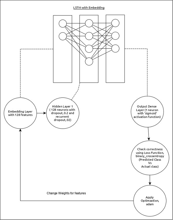
The model for the sequence analysis can be represented as below −
The core features of the model are as follows −
Input layer using Embedding layer with 128 features.
First layer, Dense consists of 128 units with normal dropout and recurrent dropout set to 0.2.
Output layer, Dense consists of 1 unit and ‘sigmoid’ activation function.
Use binary_crossentropy as loss function.
Use adam as Optimizer.
Use accuracy as metrics.
Use 32 as batch size.
Use 15 as epochs.
Use 80 as the maximum length of the word.
Use 2000 as the maximum number of word in a given sentence.
Step 1: Import the modules
Let us import the necessary modules.
from keras.preprocessing import sequence
from keras.models import Sequential
from keras.layers import Dense, Embedding
from keras.layers import LSTM
from keras.datasets import imdb
sequence.pad_sequences convert the list of input data with shape, (data) into 2D NumPy array of shape (data, timesteps). Basically, it adds timesteps concept into the given data. It generates the timesteps of length, maxlen.
In this chapter, let us write a simple MPL based ANN to do regression prediction. Till now, we have only done the classification based prediction. Now, we will try to predict the next possible value by analyzing the previous (continuous) values and its influencing factors.
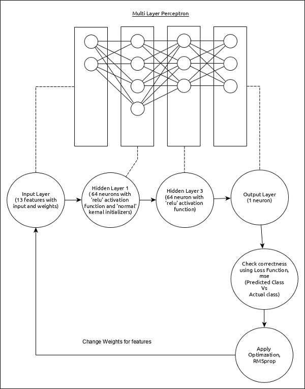
The Regression MPL can be represented as below −
The core features of the model are as follows −
Input layer consists of (13,) values.
First layer, Dense consists of 64 units and ‘relu’ activation function with ‘normal’ kernel initializer.
Second layer, Dense consists of 64 units and ‘relu’ activation function.
Output layer, Dense consists of 1 unit.
Use mse as loss function.
Use RMSprop as Optimizer.
Use accuracy as metrics.
Use 128 as batch size.
Use 500 as epochs.
Step 1 − Import the modules
Let us import the necessary modules.
import keras

from keras.datasets import boston_housing
from keras.models import Sequential
from keras.layers import Dense
from keras.optimizers import RMSprop
from keras.callbacks import EarlyStopping
from sklearn import preprocessing
from sklearn.preprocessing import scale
Here, we have normalized the training data using sklearn.preprocessing.scale function. preprocessing.StandardScaler().fit function returns a scalar with the normalized mean and standard deviation of the training data, which we can apply to the test data using scalar.transform function. This will normalize the test data as well with the same setting as that of training data.
Here, we have used callback function, EarlyStopping. The purpose of this callback is to monitor the loss value during each epoch and compare it with previous epoch loss value to find the improvement in the training. If there is no improvement for the patience times, then the whole process will be stopped.
Executing the application will give the below information as output −
Let us modify the model from MPL to Convolution Neural Network (CNN) for our earlier digit identification problem.
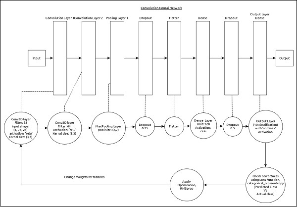
CNN can be represented as below −
The core features of the model are as follows −
Input layer consists of (1, 8, 28) values.
First layer, Conv2D consists of 32 filters and ‘relu’ activation function with kernel size, (3,3).
Second layer, Conv2D consists of 64 filters and ‘relu’ activation function with kernel size, (3,3).
Thrid layer, MaxPooling has pool size of (2, 2).
Fifth layer, Flatten is used to flatten all its input into single dimension.
Sixth layer, Dense consists of 128 neurons and ‘relu’ activation function.
Seventh layer, Dropout has 0.5 as its value.
Eighth and final layer consists of 10 neurons and ‘softmax’ activation function.
Use categorical_crossentropy as loss function.
Use Adadelta() as Optimizer.
Use accuracy as metrics.
Use 128 as batch size.
Use 20 as epochs.
Step 1 − Import the modules
Let us import the necessary modules.
import keras
from keras.datasets import mnist
from keras.models import Sequential
from keras.layers import Dense, Dropout, Flatten
from keras.layers import Conv2D, MaxPooling2D
from keras import backend as K
import numpy as np
This chapter deals with the model evaluation and model prediction in Keras.
Let us begin by understanding the model evaluation.
Model Evaluation
Evaluation is a process during development of the model to check whether the model is best fit for the given problem and corresponding data. Keras model provides a function, evaluate which does the evaluation of the model. It has three main arguments,
Test data
Test data label
verbose – true or false
Let us evaluate the model, which we created in the previous chapter using test data.
Executing the above code will output the below information.
0
The test accuracy is 98.28%. We have created a best model to identify the handwriting digits. On the positive side, we can still scope to improve our model.
Model Prediction
Prediction is the final step and our expected outcome of the model generation. Keras provides a method, predict to get the prediction of the trained model. The signature of the predict method is as follows,
Here, all arguments are optional except the first argument, which refers the unknown input data. The shape should be maintained to get the proper prediction.
Let us do prediction for our MPL model created in previous chapter using below code −
pred = model.predict(x_test)
pred = np.argmax(pred, axis = 1)[:5]
label = np.argmax(y_test,axis = 1)[:5]

print(pred)
print(label)
Here,
Line 1 call the predict function using test data.
Line 2 gets the first five prediction
Line 3 gets the first five labels of the test data.
Line 5 – 6 prints the prediction and actual label.
The output of the above application is as follows −
[7 2 1 0 4]
[7 2 1 0 4]
The output of both array is identical and it indicate that our model predicts correctly the first five images.
Previously, we studied the basics of how to create model using Sequential and Functional API. This chapter explains about how to compile the model. The compilation is the final step in creating a model. Once the compilation is done, we can move on to training phase.
Let us learn few concepts required to better understand the compilation process.
Loss
In machine learning, Loss function is used to find error or deviation in the learning process. Keras requires loss function during model compilation process.
Keras provides quite a few loss function in the losses module and they are as follows −
mean_squared_error
mean_absolute_error
mean_absolute_percentage_error
mean_squared_logarithmic_error
squared_hinge
hinge
categorical_hinge
logcosh
huber_loss
categorical_crossentropy
sparse_categorical_crossentropy
binary_crossentropy
kullback_leibler_divergence
poisson
cosine_proximity
is_categorical_crossentropy
All above loss function accepts two arguments −
y_true − true labels as tensors
y_pred − prediction with same shape as y_true
Import the losses module before using loss function as specified below −
from keras import losses
Optimizer
In machine learning, Optimization is an important process which optimize the input weights by comparing the prediction and the loss function. Keras provides quite a few optimizer as a module, optimizers and they are as follows:
Import the optimizers module before using optimizers as specified below −
from keras import optimizers
Explore our latest online courses and learn new skills at your own pace. Enroll and become a certified expert to boost your career.
Metrics
In machine learning, Metrics is used to evaluate the performance of your model. It is similar to loss function, but not used in training process. Keras provides quite a few metrics as a module, metrics and they are as follows
accuracy
binary_accuracy
categorical_accuracy
sparse_categorical_accuracy
top_k_categorical_accuracy
sparse_top_k_categorical_accuracy
cosine_proximity
clone_metric
Similar to loss function, metrics also accepts below two arguments −
y_true − true labels as tensors
y_pred − prediction with same shape as y_true
Import the metrics module before using metrics as specified below −
from keras import metrics
Compile the model
Keras model provides a method, compile() to compile the model. The argument and default value of the compile() method is as follows
from keras import losses
from keras import optimizers
from keras import metrics

model.compile(loss = 'mean_squared_error',
   optimizer = 'sgd', metrics = [metrics.categorical_accuracy])
where,
loss function is set as mean_squared_error
optimizer is set as sgd
metrics is set as metrics.categorical_accuracy
Model Training
Models are trained by NumPy arrays using fit(). The main purpose of this fit function is used to evaluate your model on training. This can be also used for graphing model performance. It has the following syntax −
model.fit(X, y, epochs = , batch_size = )
Here,
X, y − It is a tuple to evaluate your data.
epochs − no of times the model is needed to be evaluated during training.
batch_size − training instances.
Let us take a simple example of numpy random data to use this concept.
Create data
Let us create a random data using numpy for x and y with the help of below mentioned command −
import numpy as np

x_train = np.random.random((100,4,8))
y_train = np.random.random((100,10))
We have learned to create, compile and train the Keras models.
Let us apply our learning and create a simple MPL based ANN.
Dataset module
Before creating a model, we need to choose a problem, need to collect the required data and convert the data to NumPy array. Once data is collected, we can prepare the model and train it by using the collected data. Data collection is one of the most difficult phase of machine learning. Keras provides a special module, datasets to download the online machine learning data for training purposes. It fetches the data from online server, process the data and return the data as training and test set. Let us check the data provided by Keras dataset module. The data available in the module are as follows,
CIFAR10 small image classification
CIFAR100 small image classification
IMDB Movie reviews sentiment classification
Reuters newswire topics classification
MNIST database of handwritten digits
Fashion-MNIST database of fashion articles
Boston housing price regression dataset
Let us use the MNIST database of handwritten digits (or minst) as our input. minst is a collection of 60,000, 28×28 grayscale images. It contains 10 digits. It also contains 10,000 test images.
Below code can be used to load the dataset −
from keras.datasets import mnist

(x_train, y_train), (x_test, y_test) = mnist.load_data()
where
Line 1 imports minst from the keras dataset module.
Line 3 calls the load_data function, which will fetch the data from online server and return the data as 2 tuples, First tuple, (x_train, y_train) represent the training data with shape, (number_sample, 28, 28) and its digit label with shape, (number_samples, ). Second tuple, (x_test, y_test) represent test data with same shape.
Other dataset can also be fetched using similar API and every API returns similar data as well except the shape of the data. The shape of the data depends on the type of data.
Create a model
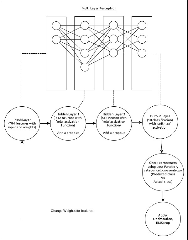
Let us choose a simple multi-layer perceptron (MLP) as represented below and try to create the model using Keras.
The core features of the model are as follows −
Input layer consists of 784 values (28 x 28 = 784).
First hidden layer, Dense consists of 512 neurons and ‘relu’ activation function.
Second hidden layer, Dropout has 0.2 as its value.
Third hidden layer, again Dense consists of 512 neurons and ‘relu’ activation function.
Fourth hidden layer, Dropout has 0.2 as its value.
Fifth and final layer consists of 10 neurons and ‘softmax’ activation function.
Use categorical_crossentropy as loss function.
Use RMSprop() as Optimizer.
Use accuracy as metrics.
Use 128 as batch size.
Use 20 as epochs.
Step 1 − Import the modules
Let us import the necessary modules.
import keras
from keras.datasets import mnist
from keras.models import Sequential
from keras.layers import Dense, Dropout
from keras.optimizers import RMSprop
import numpy as np
We have created the model, loaded the data and also trained the data to the model. We still need to evaluate the model and predict output for unknown input, which we learn in upcoming chapter.
As learned earlier, Keras model represents the actual neural network model. Keras provides a two mode to create the model, simple and easy to use Sequential API as well as more flexible and advanced Functional API. Let us learn now to create model using both Sequential and Functional API in this chapter.
Sequential
The core idea of Sequential API is simply arranging the Keras layers in a sequential order and so, it is called Sequential API. Most of the ANN also has layers in sequential order and the data flows from one layer to another layer in the given order until the data finally reaches the output layer.
A ANN model can be created by simply calling Sequential() API as specified below −
from keras.models import Sequential
model = Sequential()
Add layers
To add a layer, simply create a layer using Keras layer API and then pass the layer through add() function as specified below −
model_from_yaml() − Accepts yaml representation of the model and create a new model.
from keras.models import model_from_yaml
new_model = model_from_yaml(yaml_string)
Summarise the model
Understanding the model is very important phase to properly use it for training and prediction purposes. Keras provides a simple method, summary to get the full information about the model and its layers.
A summary of the model created in the previous section is as follows −
Model provides function for training, evaluation and prediction process. They are as follows −
compile − Configure the learning process of the model
fit − Train the model using the training data
evaluate − Evaluate the model using the test data
predict − Predict the results for new input.
Functional API
Sequential API is used to create models layer-by-layer. Functional API is an alternative approach of creating more complex models. Functional model, you can define multiple input or output that share layers. First, we create an instance for model and connecting to the layers to access input and output to the model. This section explains about functional model in brief.
Create a model
Import an input layer using the below module −
>>> from keras.layers import Input
Now, create an input layer specifying input dimension shape for the model using the below code −
>>> data = Input(shape=(2,3))
Define layer for the input using the below module −
>>> from keras.layers import Dense
Add Dense layer for the input using the below line of code −
Keras allows to create our own customized layer. Once a new layer is created, it can be used in any model without any restriction. Let us learn how to create new layer in this chapter.
Keras provides a base layer class, Layer which can sub-classed to create our own customized layer. Let us create a simple layer which will find weight based on normal distribution and then do the basic computation of finding the summation of the product of input and its weight during training.
Step 1: Import the necessary module
First, let us import the necessary modules −
from keras import backend as K
from keras.layers import Layer
Here,
backend is used to access the dot function.
Layer is the base class and we will be sub-classing it to create our layer
Step 2: Define a layer class
Let us create a new class, MyCustomLayer by sub-classing Layer class −
class MyCustomLayer(Layer):
   ...
Step 3: Initialize the layer class
Let us initialize our new class as specified below −
Line 3 calls the base or super layer’s init function.
Step 4: Implement build method
build is the main method and its only purpose is to build the layer properly. It can do anything related to the inner working of the layer. Once the custom functionality is done, we can call the base class build function. Our custom build function is as follows −
Line 1 defines the build method with one argument, input_shape. Shape of the input data is referred by input_shape.
Line 2 creates the weight corresponding to input shape and set it in the kernel. It is our custom functionality of the layer. It creates the weight using ‘normal’ initializer.
Line 6 calls the base class, build method.
Step 5: Implement call method
call method does the exact working of the layer during training process.
self.add_weight(name = 'kernel',
shape = (input_shape[1], self.output_dim),
initializer = 'normal', trainable = True)
super(MyCustomLayer, self).build(input_shape) #
Be sure to call this at the end