Category: 09. Indexing and Hashing

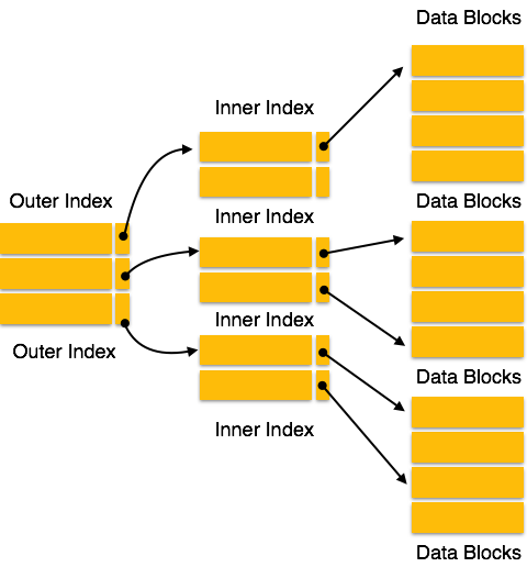
For a huge database structure, it can be almost next to impossible to search all the index values through all its level and then reach the destination data block to retrieve the desired data. Hashing is an effective technique to calculate the direct location of a data record on the disk without using index structure.

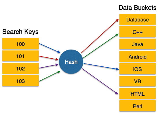
Hashing uses hash functions with search keys as parameters to generate the address of a data record.

Hash Organization

• Bucket − A hash file stores data in bucket format. Bucket is considered a unit of storage. A bucket typically stores one complete disk block, which in turn can store one or more records.
• Hash Function − A hash function, h, is a mapping function that maps all the set of search-keys K to the address where actual records are placed. It is a function from search keys to bucket addresses.

Static Hashing

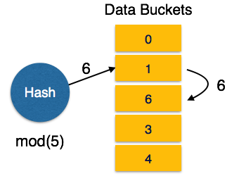
In static hashing, when a search-key value is provided, the hash function always computes the same address. For example, if mod-4 hash function is used, then it shall generate only 5 values. The output address shall always be same for that function. The number of buckets provided remains unchanged at all times.

Operation

• Insertion − When a record is required to be entered using static hash, the hash function h computes the bucket address for search key K, where the record will be stored.Bucket address = h(K)
• Search − When a record needs to be retrieved, the same hash function can be used to retrieve the address of the bucket where the data is stored.
• Delete − This is simply a search followed by a deletion operation.

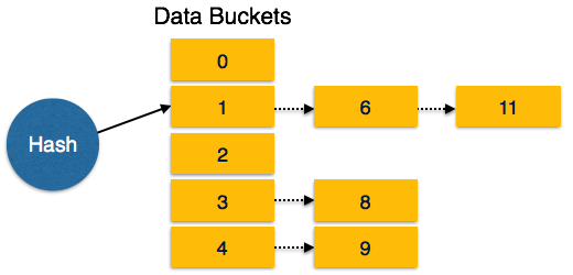
Bucket Overflow

The condition of bucket-overflow is known as collision. This is a fatal state for any static hash function. In this case, overflow chaining can be used.

• Overflow Chaining − When buckets are full, a new bucket is allocated for the same hash result and is linked after the previous one. This mechanism is called Closed Hashing.

• Linear Probing − When a hash function generates an address at which data is already stored, the next free bucket is allocated to it. This mechanism is called Open Hashing.

Dynamic Hashing

The problem with static hashing is that it does not expand or shrink dynamically as the size of the database grows or shrinks. Dynamic hashing provides a mechanism in which data buckets are added and removed dynamically and on-demand. Dynamic hashing is also known as extended hashing.

Hash function, in dynamic hashing, is made to produce a large number of values and only a few are used initially.

Organization

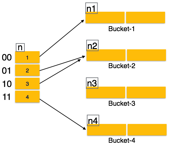
The prefix of an entire hash value is taken as a hash index. Only a portion of the hash value is used for computing bucket addresses. Every hash index has a depth value to signify how many bits are used for computing a hash function. These bits can address 2n buckets. When all these bits are consumed − that is, when all the buckets are full − then the depth value is increased linearly and twice the buckets are allocated.

Operation

• Querying − Look at the depth value of the hash index and use those bits to compute the bucket address.
• Update − Perform a query as above and update the data.
• Deletion − Perform a query to locate the desired data and delete the same.
• Insertion − Compute the address of the bucket
  • If the bucket is already full.
    • Add more buckets.
    • Add additional bits to the hash value.
    • Re-compute the hash function.
  • Else
    • Add data to the bucket,
  • If all the buckets are full, perform the remedies of static hashing.

Hashing is not favorable when the data is organized in some ordering and the queries require a range of data. When data is discrete and random, hash performs the best.

Hashing algorithms have high complexity than indexing. All hash operations are done in constant time.

Large databases require efficient methods for indexing. It is crucial that we maintain proper indexes to search records in large databases. A common challenge is to make sure the index structure remains balanced when new records are inserted or existing ones are deleted. For this purpose, there are different methods like single level indexing, multi-level indexing, and dynamic multilevel indexing.

Multilevel indexing can be done using B-Trees and B+ Trees. These advanced data structures adjust themselves automatically, keeping the operations smooth and fast. Read this chapter to learn the fundamentals of dynamic multilevel indexing and understand how B-Trees and B+ Trees work.

What is Dynamic Multilevel Indexing?

Dynamic multilevel indexing helps in maintaining an efficient search structure. This is true even when the records in a database keep changing frequently. Unlike static indexing where we can update by rebuilding the index, dynamic indexing updates itself on the fly.

The two most common structures used are B- Trees and B+ Trees. Both work as balanced tree structures. These trees keep the search times short by minimizing the number of levels. They handle insertions, deletions, and searches efficiently, even in large datasets.

The Role of B- Trees in Dynamic Indexing

A B- Tree is a balanced search tree where records are stored within its nodes. Each node contains multiple key values and pointers to other nodes or records. The key idea is to keep the tree balanced by splitting and merging the nodes as records are inserted or deleted.

How Does a B- Tree Work?

Let’s understand how a B-Tree works −

• Nodes and Keys − Each node can have several keys and pointers that form a multi-way search tree.
• Balanced Structure − The tree is always balanced, which means every leaf node is at the same level.
• Search Process − The search begins at the root and follows pointers based on key comparisons until the desired record is found.

The following image depicts how a B-Tree looks like −

Key Properties of B-Trees

Given below are some of the important properties of B-Trees −

• Every internal node can have up to “p – 1” keys and “p” pointers. Here, “p” is the order of the B-Tree.
• Keys in each node are arranged in ascending order.
• Each node must be at least half full, except for the root.
• Leaf nodes are linked for easier traversal if needed.

Example of a B-Tree

Let’s see an example of a B-Tree for a database with order and fan-out −

• Order (p) − 23 (maximum keys a node can hold)
• Fan-out (fo) − 16 (average number of pointers in a node)

We start with the root node that holds 15 key entries and 16 pointers. As new records are inserted, the tree grows as follows −

• Level 0 (Root) − 1 node with 15 keys and 16 pointers
• Level 1 − 16 nodes with 240 keys and 256 pointers
• Level 2 − 256 nodes with 3840 keys and 4096 pointers
• Level 3 (Leaf Level) − 4096 nodes holding 61,440 keys

The tree can efficiently organize over 65,535 records and we can see that there are just three levels. It is this efficiency that reduces the search times to a great extent.

B+ Trees: More Efficient than B-Tree

A B+ Tree is a modified version of a B-Tree. B+ Trees are specifically designed for indexing. In a B+ Tree, all the data records are stored only at the leaf nodes and the internal nodes hold only keys and pointers. This design allows the internal nodes to hold more keys, making the structure shallower and more efficient.

How Do B+ Trees Work

In a B+ Tree,

• Leaf Nodes − Contain records or pointers to records.
• Internal Nodes − Contain only keys and pointers to lower-level nodes.
• Linked Leaf Nodes − Leaf nodes are linked, which makes the sequential access easier.

Key Properties of B+ Trees

Listed below are some of the important properties of B+ Trees −

• Every internal node can have up to p pointers and p-1 keys.
• Leaf nodes hold actual data or pointers to data.
• Leaf nodes are linked for easy traversal.
• The tree stays balanced due to automatic splitting and merging during updates.

Example of a B+ Tree

Let us see the same example that we used for explaining B-Trees but this time, with B+ Tree logic −

Assumptions −

• Key size − 9 bytes
• Pointer size − 7 bytes (for records), 6 bytes (for blocks)
• Block size − 512 bytes

Internal Nodes − Maximum of 34 keys and 35 pointers (calculated based on available space).

Leaf Nodes − Maximum of 31 data entries (keys and data pointers).

• Root Node − 1 node with 22 keys and 23 pointers.
• Level 1 − 23 nodes holding 506 keys and 529 pointers.
• Level 2 − 529 nodes holding 11,638 keys and 12,167 pointers.
• Leaf Level − 12,167 nodes holding 255,507 data pointers.

This structure is useful and it can handle over 255,507 records efficiently with just three levels. This is why B+ Trees are commonly used in database indexing systems.

Advantages of Dynamic Multilevel Indexing

Dynamic multilevel indexing offers several advantages as given below −

• Automatic Balancing − Trees adjust themselves during insertions and deletions.
• Efficient Searches − Shallow trees mean fewer levels to search through.
• Faster Updates − Data changes are quick due to rebalancing logic.
• Scalability − B-Trees and B+ Trees handle massive datasets without performance drops.

Real-world Applications of B-Trees and B+ Trees

B-Trees and B+ Trees are widely used in −

• DBMS − For indexing large tables.
• File Systems − To manage files in storage systems.
• Search Engines − To keep search indexes optimized.
• Operating Systems − For directory management.

Difference between B-Trees and B+ Trees

The following table highlights the major differences between B-Trees and B+ Trees −

Feature	B- Tree	B+ Tree
Data Storage	In all nodes	Only in leaf nodes
Data Retrieval	Slower for range queries	Faster due to linked leaf nodes
Tree Depth	Deeper	Shallower
Use Cases	General indexing	Indexing with range queries

Data retrieval is the process in database management systems where we need speed and efficiency. We implement the concept of indexing in order to reduce the search time and facilitate faster data retrieval. As databases grow in size, efficient indexing techniques become our primary option to reduce search times. Multi-level indexing is one such indexing technique that is designed to manage large datasets with minimal disk access. Read this chapter to get a good understanding of what multi-level indexing means, what is its structure, and how it works.

What is Multi-level Indexing in DBMS?

In database systems, indexing improves the data retrieval speed by organizing the records in a way that allows faster searches. A single-level index makes a list of key values pointing to corresponding records. This process can be used with a binary search. However, when we are working with massive datasets, a single-level index becomes inefficient due to its size. This is where multi-level indexing is needed for efficiency.

Why Do We Use Multi-level Indexing?

The main reason for using multi-level indexing is to reduce the number of blocks accessed during a search. We know we can apply the binary search where the search space is divided in half at each step. Binary search requires approximately log₂ (b_i) block accesses for an index with b_i blocks. With multi-level indexing, we can improve the search speed by dividing the search space into larger segments. It will reduce the search time exponentially.

For example, instead of cutting the search space in half, we can use multi-level indexing to split it further. This reduces the search space by a factor equal to the fan-out (f₀) value, which denotes the number of entries that can fit into a single block. When the fan-out value is much larger than 2, the search process becomes significantly faster.

Structure of Multi-level Indexing

To understand the concept of multi-level indexing, we must know its structures. It is organized into different levels, each representing a progressively smaller index until a manageable size is reached.

The structure consists of −

• First Level (Base Level) − This level stores the main index entries. This is also called the base index. It contains unique key values and pointers to corresponding records.
• Second Level − This level acts as a primary index for the first level. It stores pointers to the blocks of the first level.
• Higher Levels − If the second level becomes too large to fit in a single block, then additional levels are created. It reduces the index size further.

How Does Multi-level Indexing Work?

Each level of the multi-level index reduces the number of entries in the previous level. This is done by the fan-out value (f₀). The process continues until the final level fits into a single block, referred to as the top level.

The number of levels (t) required is calculated as −

t=[logf0(r1)]

Where, r₁ is the number of entries in the first level and f₀ is the fan-out value.

From this, it is evident that searching involves retrieving a block from each level and finally accessing the data block. It results in a total of t + 1 block accesses.

Example of Multi-level Indexing

Let us take a detailed example to understand multi-level indexing in action.

The given data is as follows −

• Blocking factor (bfri) − 68 entries per block (also called the fan-out, fo).
• First-level blocks (b1) − 442 blocks.

Step 1: Calculate the Second Level

We calculate the number of blocks needed at the second level −

b2=[b1f0]=[44268]=7

The second level has seven blocks.

Step 2: Calculate the Third Level

Similarly, we can calculate the number of blocks needed at the third level −

b3=[b2f0]=[768]=1

Since the third level fits into one block, it becomes the top level of the index. This is making the total number of levels t = 3.

Step 3: Record Search Example

After making the index, we must search from it. To search for a record using this multi-level index, we need to access −

• One block from each level − Three levels in total.
• One data block from the file − The block containing the record.

Total Block Accesses is: T + 1 = 3 + 1 = 4. This is a significant improvement over a single-level index. There are 10 block accesses would have been needed using a binary search.

Types of Multi-level Indexing

Depending on the type of records and access patterns, multi-level indexing can be applied in various forms −

• Primary Index − Built on a sorted key field, which makes it sparse (only one index entry per block).
• Clustering Index − Built on non-key fields where multiple records share the same value.
• Secondary Index − Built on unsorted fields, requiring more maintenance but offering flexibility.

Indexed Sequential Access Method (ISAM)

Indexed Sequential Access Method (ISAM) is a practical implementation of multi-level indexing. ISAM is commonly used in older IBM systems. It uses a two-level index −

• Cylinder Index − Points to track-level blocks.
• Track Index − Points to specific tracks in the cylinder.

Data insertion is managed using overflow files. This is periodically merged with the main file during reorganization.

Advantages of Multi-level Indexing

Multi-level indexing offers the following benefits −

• Faster Searches − Reduces the number of disk accesses.
• Scalability − Handles large datasets efficiently.
• Supports Different Index Types − Works with primary, clustering, and secondary indexes.
• Balanced Access − Ensures near-uniform access times.

One of the major challenges in managing multi-level indexes is during insertions or deletions. It can be complex, as all index levels must be updated. This process becomes problematic when frequent updates occur.

The solution could be dynamic indexing. To address this problem, modern databases use dynamic multi-level indexes such as B − trees and B+ − trees. These structures balance the index by reorganizing the nodes automatically during insertions and deletions.

We know that data is stored in the form of records. Every record has a key field, which helps it to be recognized uniquely.

Indexing is a data structure technique to efficiently retrieve records from the database files based on some attributes on which the indexing has been done. Indexing in database systems is similar to what we see in books.

Indexing is defined based on its indexing attributes. Indexing can be of the following types −

• Primary Index − Primary index is defined on an ordered data file. The data file is ordered on a key field. The key field is generally the primary key of the relation.
• Secondary Index − Secondary index may be generated from a field which is a candidate key and has a unique value in every record, or a non-key with duplicate values.
• Clustering Index − Clustering index is defined on an ordered data file. The data file is ordered on a non-key field.

Ordered Indexing is of two types −

• Dense Index
• Sparse Index

Dense Index

In dense index, there is an index record for every search key value in the database. This makes searching faster but requires more space to store index records itself. Index records contain search key value and a pointer to the actual record on the disk.

Sparse Index

In sparse index, index records are not created for every search key. An index record here contains a search key and an actual pointer to the data on the disk. To search a record, we first proceed by index record and reach at the actual location of the data. If the data we are looking for is not where we directly reach by following the index, then the system starts sequential search until the desired data is found.

Multilevel Index

Index records comprise search-key values and data pointers. Multilevel index is stored on the disk along with the actual database files. As the size of the database grows, so does the size of the indices. There is an immense need to keep the index records in the main memory so as to speed up the search operations. If single-level index is used, then a large size index cannot be kept in memory which leads to multiple disk accesses.

Multi-level Index helps in breaking down the index into several smaller indices in order to make the outermost level so small that it can be saved in a single disk block, which can easily be accommodated anywhere in the main memory.

B⁺ Tree

A B⁺ tree is a balanced binary search tree that follows a multi-level index format. The leaf nodes of a B⁺ tree denote actual data pointers. B⁺ tree ensures that all leaf nodes remain at the same height, thus balanced. Additionally, the leaf nodes are linked using a link list; therefore, a B⁺ tree can support random access as well as sequential access.

Structure of B⁺ Tree

Every leaf node is at equal distance from the root node. A B⁺ tree is of the order n where n is fixed for every B⁺ tree.

Internal nodes −

• Internal (non-leaf) nodes contain at least ⌈n/2⌉ pointers, except the root node.
• At most, an internal node can contain n pointers.

Leaf nodes −

• Leaf nodes contain at least ⌈n/2⌉ record pointers and ⌈n/2⌉ key values.
• At most, a leaf node can contain n record pointers and n key values.
• Every leaf node contains one block pointer P to point to next leaf node and forms a linked list.

B⁺ Tree Insertion

• B⁺ trees are filled from bottom and each entry is done at the leaf node.
• If a leaf node overflows −
  • Split node into two parts.
  • Partition at i = ⌊(m+1)_/2⌋.
  • First i entries are stored in one node.
  • Rest of the entries (i+1 onwards) are moved to a new node.
  • i^th key is duplicated at the parent of the leaf.
• If a non-leaf node overflows −
  • Split node into two parts.
  • Partition the node at i = ⌈(m+1)_/2⌉.
  • Entries up to i are kept in one node.
  • Rest of the entries are moved to a new node.

B⁺ Tree Deletion

• B⁺ tree entries are deleted at the leaf nodes.
• The target entry is searched and deleted.
  • If it is an internal node, delete and replace with the entry from the left position.
• After deletion, underflow is tested,
  • If underflow occurs, distribute the entries from the nodes left to it.
• If distribution is not possible from left, then
  • Distribute from the nodes right to it.
• If distribution is not possible from left or from right, then
  • Merge the node with left and right to it.