Category: 08. Storage and File Structure

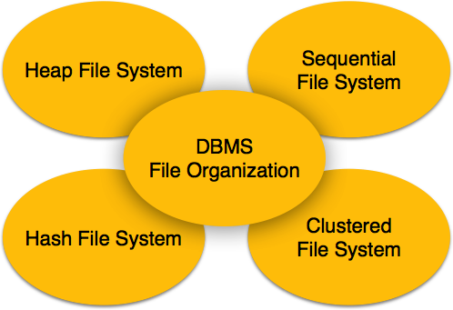
In database management, there are plenty of different techniques to store files for easy access and optimized use-cases. Two of the most common types of file organizations are unordered records (heap files) and ordered records (sorted files), each with their own strengths, weaknesses, and use cases.

Read this chapter to learn in detail the concepts of unordered and ordered files, explore their differences, and see real-world examples of how they are used.

Unordered Records: The Heap File

Unordered records or heap files are nothing but a dump. Heap files are the simplest form of file organization. The records are stored in the order they are inserted. When a new record is added, it is placed at the end of the file. This process makes the insertion quick and straightforward.

How Do Heap Files Work?

Let’s see how heap files work −

• When a record is inserted, the last disk block of the file is loaded into memory. Here the new record is appended. The block is written back to the disk.
• The address of the last block is maintained in the file header. It gives quick access for new inserts.

Advantages of Using Heap Files

Following are the advantages of using heap files −

• Quick Insertions − Adding a record is very efficient, since no sorting or restructuring is applied.
• Simplicity − The structure is straightforward and it requires minimal overhead.

Limitations of Heap Files

Heap files are simple and easy to maintain, but they have their own limitations −

• Linear Search for Retrieval − To find a specific record, we need to rely on a linear search through all blocks. On an average, half the blocks must be searched, which makes the retrieval process slow for large files.
• Wasted Space − Deleting a record leaves unused space in the block unless the file is reorganized periodically.
• Inefficient Updates − Updates such as modifying some variable-length records, deleting an old record and inserting a new one can further fragment the file.

Handling Deletions in Heap Files

One way to handle deletions in heap files is by using a deletion marker. Here, each record has a small flag (a byte or a bit) to indicate whether it is active or deleted. When a record is marked as deleted, it remains in the file but is ignored during searches. Periodically, the file is reorganized to reclaim space and remove deleted records.

Ordered Records: The Sorted File

Ordered records are sorted and organized based on the values of a specific field which is known as the ordering field. If this field is unique for each record, it is called the ordering key. This type of file organization makes searches and sequential access faster, however it comes with its challenges for insertions and deletions.

How Do Ordered Records Work?

Records are stored in ascending or descending order of the ordering field. For example, an employee database might be sorted alphabetically by employee names. The records are placed in blocks, and the blocks are organized contiguously on the disk.

Advantages of Ordered Records

Given below are some of the advantages of using ordered records −

• Efficient Searches − We can use binary search or other fast search techniques, as the system can quickly locate a record based on the ordering field. For example, if the file has 100 blocks, a binary search requires only about 7 block accesses on average.
• Easy Sequential Access − It’s easy to access ordered records since the blocks are stored contiguously.
• Sorting for Queries − Ordered records simplify certain queries, such as finding all employees whose names start with a specific letter.

Limitations of Ordered Records

While retrieval of data is efficient in ordered records, updates and modifications are not so easy. Given below are some other notable limitations of using ordered records −

• Insertion Complexity − To insert a new record, the correct position in the file must be located. It requires shifting many records to make space, which is time-consuming for large files.
• Costly Deletions − Deleting a record leaves a gap. It requires reorganization to maintain order. Using a deletion marker can delay reorganization but does not eliminate the overhead.
• Overflow Files − To address insertion delays, we can add new records and they are often stored in a temporary unordered file (overflow file). Periodically, the overflow file is merged with the main file. This is a resource-intensive process.

Example: Binary Search in a Sorted File

Imagine an ordered file of employee records, sorted by names. The file has 100 blocks. We want to find the employee named Amit Mondal. Using a binary search, we can do the following −

• The system starts with the middle block, say block 50, and checks if Amit’s name falls before or after the names in that block.
• If Amit’s name is alphabetically before, the search narrows to blocks 1–49; otherwise, it checks blocks 51–100.
• This process continues, halving the range with each step, until the record is found or all possibilities are exhausted.
• This method requires only log2(100) ≈ 7 block accesses, which is much faster than the linear search required for heap files.

Differences between Unordered and Ordered Files

The following table highlights the key differences between ordered and unordered files −

Aspect	Unordered Records (Heap Files)	Ordered Records (Sorted Files)
Insertion	Faster; new records are added to the end of the file	Slower; inserting requires finding the correct position
Search	Linear search; slow for large files	Binary search; much faster for ordering field
Deletion	Leaves gaps; periodic reorganization needed	Gaps also require reorganization, or use of overflow files
Modification	Simple for fixed-length records	Complex if ordering field changes
Sequential Access	Inefficient; requires sorting first	Very efficient due to physical ordering

Overflow Files

To speed up insertions, new records are stored in an overflow file. For example −

• The main file contains records sorted by names; the overflow file, on the other hand, holds unsorted new records.
• Periodically, the overflow file is merged with the main file, which is needed to ensure the overall file remains ordered.

External Sorting

For very large files, sorting them entirely in memory is impractical. Now external sorting techniques divide the file into smaller chunks, sort each chunk, and then merge them together. This process is quite useful and the file remains ordered without overwhelming system resources.

When to Use Unordered vs. Ordered Files

Unordered files are suitable for applications where insertions are frequent, and searches are infrequent or involve scanning the entire file (e.g., collecting log data for later analysis).

Ordered files are ideal when efficient searches based on a specific field are needed, or when sequential access is common (e.g., payroll processing by employee names).

Storing data means more than just saving it somewhere. It is about organizing the data efficiently such that the stored data can retrieved and used easily. In DBMS, it means figuring out how to place file records on a disk. Although it may seem like a simple task, it involves some clever techniques to handle different types of records. These techniques are used to save space, and make the database faster.

Read this chapter to learn how file records are placed on a disk. We will have specific examples to understand the methods used to store both fixed-length and variable-length records.

Records and File Types

A record in a DBMS is a collection of data values. We often tie them to a specific entity. Think of it like a detailed entry in a contact list. For instance, an EMPLOYEE record may have different fields such as name, employee ID, department, and salary. Each of these fields holds a piece of information about a particular employee.

Placing file records on disk enables better data indexing and searching capabilities. With an organized structure, it becomes easier to locate specific files or retrieve relevant information without wasting time and resources.

Techniques for Placing File Records on Disk

There are several techniques for placing file records on disk, including −

• Fixed-Length Records − Every record is the same size. Each field has a predetermined length, which makes it easier to locate data because the position of each field is consistent.
• Variable-Length Records − Here the records can differ in size. It happens when some fields hold varying amounts of data. For example, a name that might be 5 characters long for one person and 20 for another.

Let’s now discuss each of these techniques in detail.

Fixed-Length Records on Disk

Fixed-length records are straightforward to store because of their uniform size. The following example shows how it works −

Example of Fixed-Length Records

Suppose we have a fixed-length record for employees. It contains the following fields −

• Name − 30 characters
• Social Security Number (SSN) − 9 characters
• Salary − 4 bytes (integer)
• Job Code − 4 bytes (integer)
• Department − 20 characters

Each field’s length is fixed. If we add them up, the total record size will be (30 + 9 + 4 + 4 + 20) = 67 bytes. It is this uniformity that makes it simple to calculate where a specific field is within a record. For instance, the salary field starts at byte 39 (the first 30 bytes are for the name, followed by 9 bytes for SSN).

Limitations of Fixed-Length Records

Fixed-length records are easy to handle, but they can waste space. For example, if a department name is only 5 characters long, the remaining 15 bytes are unused. For thousands of records, this wasted space adds up.

Another issue arises with optional fields. Sometimes some records do not have values for certain fields. Space is reserved for those fields as well. Let us say not every employee has a job code. Even so, 4 bytes will be reserved for that field in every record.

Variable-Length Records on Disk

Variable-length records save space by allowing fields to take up only as much space as they need. But, how do we manage records when their sizes are unpredictable?

Using Separators − We can use separator characters like pipe (|) to separate the fields in a record. So, a record might look like this:

Smith|123456789|45000|Computer Department|

Separators make it clear where each field ends, even if the field sizes vary. This format works well but requires extra processing to find the data.

Storing Field Lengths − Another method is to store the length of each field at the beginning of the record. For example,

30 Smith	9123456789645000

Here, the numbers before each field indicate its size. This system reads the length, then grabs the corresponding number of bytes.

Practical Example: Handling Optional Fields

Let us say our EMPLOYEE records include an optional field for a middle name. For some employees, this field may be empty. With variable-length records, we can save space by only including the field when it has a value.

In a file with such records −

• Record A − Smith|123456789|45000|Computer Department|
• Record B − Jones|987654321|52000|HR|Michael

In Record A, the middle name is skipped. This flexibility makes variable-length records more space-efficient, however it complicates how records are processed.

Mixed Records and Real-Life Applications

Sometimes, files contain a mix of record types. If we consider a university database with two types of records −

• Student Records − Fields for name, ID, courses, and grades.
• Course Records − Fields for course name, instructor, and schedule.

If related student and course records are stored together, their sizes will vary. This is common in real-world databases where different entities need to be linked efficiently.

Example of Mixed Records

In one block, we might have −

• Student Record − John Doe|12345|Math: A, History: B|
• Course Record − Math|Prof. Smith|MWF 10:00 AM|

The database system keeps track of the record type and adjusts accordingly.

Organization of Records on Disk

When records are placed on a disk, they are grouped into blocks. Blocks are small chunks of data that the disk reads and writes. The way the records are packed into blocks affects the performance.

• Unspanned Records − In this method, a record must fit entirely within one block. If a block has extra space left after storing several records, that space remains unused. This approach is simple but wastes some disk space.
• Spanned Records − For larger records, the spanned approach allows a single record to stretch across multiple blocks. Here, the pointer at the end of one block tells the system where the rest of the record is stored. This method is more space-efficient but slightly more complex to handle in real life scenario.

Example: Spanned vs. Unspanned

Take a look at the following examples of spanned and unspanned records −

• Unspanned Block − Record 1 | Record 2 | Record 3 | Empty Space
• Spanned Block − Record 1 | Part of Record 2 (next block has the rest of Record 2)

Optimizing Record Placement

We need to optimize the placement of records to best utilize the disk space and improve the speed. For example, if an employee’s records are frequently accessed alongside their department details, these can be placed on the same block.

There is another type of optimization called indexing. By creating an index that points to the location of records, the system reduces the time it takes to find specific data.

Efficient data handling techniques in DBMS ensure that operations like reading and writing data are fast and reliable. Buffers and disk blocks play an important role in efficient data handling by bridging the gap between the slower secondary storage devices and the faster main memory. Read this chapter to learn the basic concepts of buffering and disk blocks, and how they work together in data base management.

Buffering in DBMS

A buffer is a temporary holding area in memory where the data is placed before it is processed or written to the disk. Buffering is a technique used to manage the transfer of data between the slower secondary storage and the faster main memory. This process increases the processing speed by capitalizing on the difference in speed between these storage layers.

Importance of Buffering

As an analogy of buffering, imagine you are pouring water from a large jug into a small glass. You cannot pour it all at once. The buffer works in a similar way and ensures that the data flows smoothly without overwhelming the system.

Data transfer in a DBMS is not instantaneous. Buffering helps by allowing the system to overlap data processing and transfer operations. While one buffer is being filled with new data from the disk, another buffer can be processed by the CPU. This simple method significantly boosts the efficiency of the system.

What is Double Buffering?

In double buffering, two buffers are used alternately. While one is being filled, the other is being processed. This process shows that the CPU is never idle, waiting for data.

Let us see an example to make it more relatable. Consider a conveyor belt in a factory. While one worker loads the goods onto the belt, another worker packs them. They work simultaneously to keep the process smoothly running. Similarly, double buffering allows the CPU and disk I/O operations to run in parallel.

In the context of DBMS −

• A disk block is read from the secondary storage and placed in buffer A.
• While buffer A is being processed by the CPU, buffer B is filled with the next block of data.
• The process continues alternately, minimizing the time the CPU spends waiting for data.

This method is particularly useful for reading a continuous stream of data blocks from the disk.

Concepts of Disk Blocks

The data in secondary storage is stored in units known as blocks. A block is the smallest unit of data transfer between the disk and the memory. Each block can hold multiple records. The size of a block is typically fixed during disk formatting.

Instead of transferring one record at a time, we use blocks of data that group several records together. This process reduces the number of I/O operations and thereby improves the overall data transfer efficiency. It is like buying groceries in bulk rather than making multiple trips to the store for individual items. Buying in bulk saves both time and effort.

Buffering and Blocks in Action

When blocks of data are transferred from the disk to the main memory, they are placed in buffers for processing. To understand this, let us see how we can use two buffers, A and B −

• Data from the disk is read into buffer A.
• While the CPU processes data in A, the next block is read into buffer B.
• As soon as the CPU finishes processing A, it moves to B, and the next block is loaded into A.

Let’s elaborate this overlapping operation with a practical example. Suppose the time required to process a block in memory is less than the time needed to read the next block from the disk. By using two buffers −

• The CPU can start processing data as soon as the first block is transferred to memory.
• Next, the disk I/O system prepares the next block in the second buffer.

This process avoids delays, because the CPU does not have to wait for the next block to be read. This technique keeps both the CPU and disk busy, making the process more efficient.

Advantages of Buffering

Buffering in DBMS offers several benefits, including the following −

• Reduced Waiting Time − In overlapping operations, buffering minimizes the time the CPU spends waiting for data.
• Continuous Data Flow − Double buffering allows data to be processed and transferred seamlessly.
• Improved Performance − The system can handle larger workloads without slowing down. Buffering also ensures the tasks are distributed more effectively.

Limitations of Buffering

Buffering also has its limitations, which are listed below −

• Complexity − Implementing buffering mechanisms like double buffering requires careful management to avoid errors.
• Memory Usage − Buffers take up space in the main memory, which could be a limitation for systems with restricted memory capacity.
• Varied Workloads − In cases where data access patterns are unpredictable, buffering might not always deliver optimal performance.

Real-World Applications of Buffering

Buffers and blocks play an important role in applications where large volumes of data need to be processed efficiently. For example −

• Online Databases − Systems like e-commerce platforms rely on buffering to handle millions of user queries and transactions without delays.
• Data Analytics − Blocks and buffering techniques enable us to process huge datasets quickly.
• Backup Operations − During database backups, buffering ensures that the data is written to storage devices in an organized manner.

Buffering and blocks are also used in video streaming services, where buffering gives uninterrupted playback experience by loading data in advance.

Databases handle huge volumes of data that must be stored efficiently and accessed reliably. Database management systems use the primary memory (RAM) for generating speed while handling active operations, however RAMs are volatile and costly for large datasets. This is where the secondary storage devices come into the picture.

Secondary storage devices are non-volatile, provide higher capacities, and are quite cost-effective. These devices are essential for long-term data storage in DBMS. Read this chapter to get a good understanding of the types of secondary storage devices used in DBMS.

Secondary Storage Devices for Databases

For databases, we need stable storages. Secondary storage devices store data persistently. They are slower than primary memory but offer significantly larger storage capacities and are more affordable per byte. Data stored in secondary storage remains intact even when the system is turned off, ensuring data permanence.

Common secondary storage devices are mainly of two types â€“ magnetic disks and magnetic tapes. Both these types of secondary storage devices have different use cases based on their performance and accessibility features.

Magnetic Disks

Magnetic Disks or Hard Disk Drives (HDD) are one of the most commonly used storage devices in DBMS. These devices are used for both personal and enterprise systems as they provide a perfect balance of performance, durability, and cost.

How Do Magnetic Disks Work?

Magnetic disks are circular plates coated with a magnetic material. Data is stored on these plates by magnetizing the areas on the disk that represent binary values of “0” or “1”. Modern magnetic disks typically come in either single-sided or double-sided formats. Single-sided disks store data on one surface, while double-sided disks utilize both the surfaces for higher storage capacity.

Data Organization on Disks

The structure of magnetic disks is specially designed to maximize storage and facilitate fast access. Disks have three major parts that we need to consider −

• Tracks − Concentric circles on the surface of the disk where data is stored.
• Sectors − Divisions of a track that hold a fixed amount of data, usually 512 to 8192 bytes.
• Cylinders − Groups of tracks with the same diameter across multiple platters. Cylinders allow for faster data retrieval as the read/write head doesn’t need to move between tracks.

A modern magnetic disk might implement Zone Bit Recording (ZBR). Here the tracks in different zones have varying numbers of sectors. This optimization techniques allows for higher storage density in the outer tracks without compromising performance.

Advantages of Magnetic Disks

Following are the advantages of using magnetic disks −

• Random Access − Magnetic disks, unlike sequential storage, allow direct access to specific data blocks, which makes them highly efficient for databases.
• High Capacity − Disks can store terabytes of data. They are suitable for modern applications with large datasets.
• Durability − Magnetic disks are designed to withstand repeated read and write operations.

Performance Example: Seagate Cheetah Disk

The Seagate Cheetah 15K.6 is a high-performance magnetic disk that illustrates the capabilities of modern storage. With a formatted capacity of 450 GB and rotational speeds of 15,000 rpm, it achieves an internal transfer rate of up to 2225 Mb/sec. Its average seek time is 3.4 ms for read operations, which makes it ideal for enterprise-level DBMS where speed is critical.

Magnetic Tape Storage: A Reliable Backup Solution

Magnetic tapes are another category of secondary storage devices. These devices are not so popular now, however they still remain indispensable for archival and backup purposes.

How Do Magnetic Tapes Work?

Magnetic tapes are sequential storage devices. Here the data is stored on long strips of magnetic material wound onto reels or cartridges. Accessing the data stored on magnetic tapes means scanning through previous blocks to reach the desired one. It is this property of sequential access that makes the tapes slower than disks for random data retrieval.

Characteristics of Magnetic Tapes

Given below are some of the important characteristics of magnetic tapes −

• High Storage Capacity − Modern magnetic tapes can store a very large volume of data, like hundreds of gigabytes per cartridge. It makes them suitable for large-scale backups.
• Cost-Effectiveness − Tapes are cheaper than disks, both in terms of initial cost and long-term storage.
• Sequential Access − Magnetic tapes are slower for specific data retrieval. They take longer time in reading or writing large continuous datasets.

Real-World Example: Sun Storage SL8500

The Sun Storage SL8500 is an example of such a magnetic tape. With a storage capacity of up to 70 petabytes and throughput rates reaching 193.2 TB/hour, this system is ideal for enterprises handling massive backups. Robotic arms and automatic labeling are used with them.

Applications of Magnetic Tapes

Given below are some of the important applications of magnetic tapes −

• Backup Storage − Tapes are essential tools for creating periodic backups of databases. They protect against disk failures and data corruption.
• Archiving − Magnetic tapes are ideal for storing and archiving historical or seldom-used data for future reference.
• Disaster Recovery − Tapes offer a reliable solution for recovering data in catastrophic scenarios.

Buffering in Secondary Storage

No doubt secondary storages have larger capacity, but their speed often lags behind that of primary memory devices. To bridge this gap, DBMS uses buffering techniques to optimize data transfer between disks and main memory.

• Double Buffering − Double buffering is a widely used technique where two buffers are alternated during data transfer. While one buffer is being filled with data from the disk, the other is processed by the CPU. This overlap ensures continuous data flow, reducing delays caused by waiting for disk operations.
• Impact on Performance − Double buffering improves the efficiency significantly when transferring multiple blocks of data. For example, when processing a database query that spans several disk blocks, the system can simultaneously read and process data, minimizing the idle time.

Access Times in Magnetic Disks

Consider the following three key steps while accessing data that is stored on magnetic disks −

• Seek Time − It’s the time taken to position the read/write head over the correct track.
• Rotational Delay − The wait for the desired sector to rotate under the read/write head.
• Block Transfer Time − The time required to move the data block from disk to memory.

Example − A disk rotating at 15,000 rpm has an average rotational delay of 2 milliseconds. Now consider with seek time and block transfer time, the total delay can range from 9 to 60 milliseconds. While this is relatively fast, it will still be slower than the speeds achievable by the primary memory.

Applications of Secondary Storage in DBMS

Secondary storage devices are crucial for several DBMS operations −

• Online Storage − Magnetic disks handle active databases that require frequent read/write operations.
• Backup and Recovery − The data stored on magnetic tapes can be restored in case of failure or corruption.
• Archival Systems − Outdated but legally required records are stored on tapes to save on costs while meeting compliance requirements.
• Scalable Storage Solutions − Large-scale systems, like storage area networks (SANs), use secondary storage for managing enterprise-level databases.

Limitations of Secondary Storage

Despite their benefits, secondary storage devices face certain limitations −

• Latency − Access times are significantly slower compared to primary memory.
• Maintenance − Tapes require regular maintenance to ensure data integrity over time.
• Costs for High Performance − While basic storage is cheap, high-performance disks like the Seagate Cheetah can be costly.

Conclusion

In this chapter, we presented in detail the role of secondary storage devices in DBMS. Starting with an overview of the importance and features of secondary storage devices, we focussed on the organization of magnetic disks, including real-world examples like the Seagate Cheetah 15K.6.

In addition, we covered the use of magnetic tapes for backup and archival purpose, highlighting systems like the Sun Storage SL8500. Thereafter, we explored the buffering techniques and how they improve the performance of secondary storage devices. We finished the chapter by highlighting the applications and limitations of secondary storage devices in DBMS.

Relative data and information is stored collectively in file formats. A file is a sequence of records stored in binary format. A disk drive is formatted into several blocks that can store records. File records are mapped onto those disk blocks.

File Organization

File Organization defines how file records are mapped onto disk blocks. We have four types of File Organization to organize file records −

Heap File Organization

When a file is created using Heap File Organization, the Operating System allocates memory area to that file without any further accounting details. File records can be placed anywhere in that memory area. It is the responsibility of the software to manage the records. Heap File does not support any ordering, sequencing, or indexing on its own.

Sequential File Organization

Every file record contains a data field (attribute) to uniquely identify that record. In sequential file organization, records are placed in the file in some sequential order based on the unique key field or search key. Practically, it is not possible to store all the records sequentially in physical form.

Hash File Organization

Hash File Organization uses Hash function computation on some fields of the records. The output of the hash function determines the location of disk block where the records are to be placed.

Clustered File Organization

Clustered file organization is not considered good for large databases. In this mechanism, related records from one or more relations are kept in the same disk block, that is, the ordering of records is not based on primary key or search key.

File Operations

Operations on database files can be broadly classified into two categories −

• Update Operations
• Retrieval Operations

Update operations change the data values by insertion, deletion, or update. Retrieval operations, on the other hand, do not alter the data but retrieve them after optional conditional filtering. In both types of operations, selection plays a significant role. Other than creation and deletion of a file, there could be several operations, which can be done on files.

• Open − A file can be opened in one of the two modes, read mode or write mode. In read mode, the operating system does not allow anyone to alter data. In other words, data is read only. Files opened in read mode can be shared among several entities. Write mode allows data modification. Files opened in write mode can be read but cannot be shared.
• Locate − Every file has a file pointer, which tells the current position where the data is to be read or written. This pointer can be adjusted accordingly. Using find (seek) operation, it can be moved forward or backward.
• Read − By default, when files are opened in read mode, the file pointer points to the beginning of the file. There are options where the user can tell the operating system where to locate the file pointer at the time of opening a file. The very next data to the file pointer is read.
• Write − User can select to open a file in write mode, which enables them to edit its contents. It can be deletion, insertion, or modification. The file pointer can be located at the time of opening or can be dynamically changed if the operating system allows to do so.
• Close − This is the most important operation from the operating systems point of view. When a request to close a file is generated, the operating system
  • removes all the locks (if in shared mode),
  • saves the data (if altered) to the secondary storage media, and
  • releases all the buffers and file handlers associated with the file.

The organization of data inside a file plays a major role here. The process to locate the file pointer to a desired record inside a file various based on whether the records are arranged sequentially or clustered.

Databases are stored in file formats, which contain records. At physical level, the actual data is stored in electromagnetic format on some device. These storage devices can be broadly categorized into three types −

• Primary Storage − The memory storage that is directly accessible to the CPU comes under this category. CPU’s internal memory (registers), fast memory (cache), and main memory (RAM) are directly accessible to the CPU, as they are all placed on the motherboard or CPU chipset. This storage is typically very small, ultra-fast, and volatile. Primary storage requires continuous power supply in order to maintain its state. In case of a power failure, all its data is lost.
• Secondary Storage − Secondary storage devices are used to store data for future use or as backup. Secondary storage includes memory devices that are not a part of the CPU chipset or motherboard, for example, magnetic disks, optical disks (DVD, CD, etc.), hard disks, flash drives, and magnetic tapes.
• Tertiary Storage − Tertiary storage is used to store huge volumes of data. Since such storage devices are external to the computer system, they are the slowest in speed. These storage devices are mostly used to take the back up of an entire system. Optical disks and magnetic tapes are widely used as tertiary storage.

Memory Hierarchy

A computer system has a well-defined hierarchy of memory. A CPU has direct access to it main memory as well as its inbuilt registers. The access time of the main memory is obviously less than the CPU speed. To minimize this speed mismatch, cache memory is introduced. Cache memory provides the fastest access time and it contains data that is most frequently accessed by the CPU.

The memory with the fastest access is the costliest one. Larger storage devices offer slow speed and they are less expensive, however they can store huge volumes of data as compared to CPU registers or cache memory.

Magnetic Disks

Hard disk drives are the most common secondary storage devices in present computer systems. These are called magnetic disks because they use the concept of magnetization to store information. Hard disks consist of metal disks coated with magnetizable material. These disks are placed vertically on a spindle. A read/write head moves in between the disks and is used to magnetize or de-magnetize the spot under it. A magnetized spot can be recognized as 0 (zero) or 1 (one).

Hard disks are formatted in a well-defined order to store data efficiently. A hard disk plate has many concentric circles on it, called tracks. Every track is further divided into sectors. A sector on a hard disk typically stores 512 bytes of data.

Redundant Array of Independent Disks

RAID or Redundant Array of Independent Disks, is a technology to connect multiple secondary storage devices and use them as a single storage media.

RAID consists of an array of disks in which multiple disks are connected together to achieve different goals. RAID levels define the use of disk arrays.

RAID 0

In this level, a striped array of disks is implemented. The data is broken down into blocks and the blocks are distributed among disks. Each disk receives a block of data to write/read in parallel. It enhances the speed and performance of the storage device. There is no parity and backup in Level 0.

RAID 1

RAID 1 uses mirroring techniques. When data is sent to a RAID controller, it sends a copy of data to all the disks in the array. RAID level 1 is also called mirroring and provides 100% redundancy in case of a failure.

RAID 2

RAID 2 records Error Correction Code using Hamming distance for its data, striped on different disks. Like level 0, each data bit in a word is recorded on a separate disk and ECC codes of the data words are stored on a different set disks. Due to its complex structure and high cost, RAID 2 is not commercially available.

RAID 3

RAID 3 stripes the data onto multiple disks. The parity bit generated for data word is stored on a different disk. This technique makes it to overcome single disk failures.

RAID 4

In this level, an entire block of data is written onto data disks and then the parity is generated and stored on a different disk. Note that level 3 uses byte-level striping, whereas level 4 uses block-level striping. Both level 3 and level 4 require at least three disks to implement RAID.

RAID 5

RAID 5 writes whole data blocks onto different disks, but the parity bits generated for data block stripe are distributed among all the data disks rather than storing them on a different dedicated disk.

RAID 6

RAID 6 is an extension of level 5. In this level, two independent parities are generated and stored in distributed fashion among multiple disks. Two parities provide additional fault tolerance. This level requires at least four disk drives to implement RAID.