Category: 04. Relational Algebra

Relational Algebra provides the theoretical foundation of querying. It is used for understanding and manipulating data in relational databases. It is used for a variety of operations to query and transform datasets effectively. By understanding these operations, database users can perform complex queries while maintaining clarity and precision.

In this chapter, we will see several query examples from relational algebra. Each example is based on a specific scenario and demonstrates the practical application of relational algebra operations such as selection, projection, join, union, and division.

Let us first take a look at the required tables and their data to express the query in true sense.

EMPLOYEE Table

Here’s the EMPLOYEE table that collects the data relevant to all employees –

Fname	Minit	Lname	Ssn	Bdate	Address	Sex	Salary	Super_ssn	Dno
John	B	Smith	123456789	1965-01-09	731 Fondren, Houston, TX	M	30000	333445555	5
Franklin	T	Wong	333445555	1955-12-08	638 Voss, Houston, TX	M	40000	888665555	5
Alicia	J	Zelaya	999887777	1968-01-19	3321 Castle, Spring, TX	F	25000	987654321	4
Jennifer	S	Wallace	987654321	1941-06-20	291 Berry, Bellaire, TX	F	43000	888665555	4
Ramesh	K	Narayan	666884444	1962-09-15	975 Fire Oak, Humble, TX	M	38000	333445555	5
Joyce	A	English	453453453	1972-07-31	5631 Rice, Houston, TX	F	25000	333445555	5
Ahmad	V	Jabbar	987987987	1969-03-29	980 Dallas, Houston, TX	M	25000	987654321	4
James	E	Borg	888665555	1937-11-10	450 Stone, Houston, TX	M	55000	NULL	1

DEPARTMENT Table

There are three departments as highlighted in the following DEPARTMENT table –

Dname	Dnumber	Mgr_ssn	Mgr_start_date
Research	5	333445555	1988-05-22
Administration	4	987654321	1995-01-01
Headquarters	1	888665555	1981-06-19

PROJECT Table

The PROJECT table contains the relevant data of all the projects –

Pname	Pnumber	Plocation	Dnum
ProductX	1	Bellaire	5
ProductY	2	Sugarland	5
ProductZ	3	Houston	5
Computerization	10	Stafford	4
Reorganization	20	Houston	1
Newbenefits	30	Stafford	4

WORKS_ON Table

The WORKS_ON table gathers which employee is working on which project for how many hours –

Essn	Pno	Hours
123456789	1	32.5
123456789	2	7.5
666884444	3	40.0
453453453	1	20.0
453453453	2	20.0
333445555	2	10.0
333445555	3	10.0
333445555	10	10.0
333445555	20	10.0
999887777	30	30.0
999887777	10	10.0
987987987	10	35.0
987987987	30	5.0
987654321	30	20.0
987654321	20	15.0
888665555	20	NULL

DEPENDENT Table

The DEPENDENT table is as follows –

Essn	Dependent_name	Sex	Bdate	Relationship
333445555	Alice	F	1986-04-05	Daughter
333445555	Theodore	M	1983-10-25	Son
333445555	Joy	F	1958-05-03	Spouse
987654321	Abner	M	1942-02-28	Spouse
123456789	Michael	M	1988-01-04	Son
123456789	Alice	F	1988-12-30	Daughter
123456789	Elizabeth	F	1967-05-05	Spouse

Query Examples on Relational Algebra

Let us now check some queries that extracts data from the inputs supplied in the above tables –

Retrieve the Name and Address of Employees in the Research Department

This query is to identify employees working in the “Research” department and retrieve their names and addresses.

Steps − Use a selection operation to filter the “Research” department from the DEPARTMENT relation –

RESEARCHDEPT←σDname=′Research′(DEPARTMENT)

Dname	Dnumber	Mgr_ssn	Mgr_start_date
Research	5	333445555	1988-05-22

Join the resulting relation with the EMPLOYEE relation using the department number (Dnumber and Dno) –

RESEARCHEMPS←RESEARCHDEPT⋈Dnumber=DnoEMPLOYEE

Dname	Dnumber	Mgr_ssn	Mgr_start_date	Fname	Minit	Lname	Ssn	Bdate	Address	Sex	Salary	Super_ssn	Dno
Research	5	333445555	1988-05-22	John	B	Smith	123456789	1965-01-09	731 Fondren, Houston, TX	M	30000	333445555	5
Research	5	333445555	1988-05-22	Franklin	T	Wong	333445555	1955-12-08	638 Voss, Houston, TX	M	40000	888665555	5
Research	5	333445555	1988-05-22	Ramesh	K	Narayan	666884444	1962-09-15	975 Fire Oak, Humble, TX	M	38000	333445555	5
Research	5	333445555	1988-05-22	Joyce	A	English	453453453	1972-07-31	5631 Rice, Houston, TX	F	25000	333445555	5

Finally, apply a projection operation to retrieve the desired attributes (first name, last name, and address).

RESULT←πFname,Lname,Address(RESEARCHEMPS)

Fname	Lname	Address
John	Smith	731 Fondren, Houston, TX
Franklin	Wong	638 Voss, Houston, TX
Ramesh	Narayan	975 Fire Oak, Humble, TX
Joyce	English	5631 Rice, Houston, TX

In-Line Expression −

πFname,Lname,Address(σDname=′Research′(DEPARTMENT⋈Dnumber=DnoEMPLOYEE))

List Project Details for Stafford

For projects located in “Stafford,” we are going to retrieve the project number, the controlling department, and the manager’s details (last name, address, and birth date).

Steps − Filter projects located in “Stafford” using selection.

STAFFORD_PROJS←σPlocation=′Stafford′(PROJECT)

Pname	Pnumber	Plocation	Dnum
Computerization	10	Stafford	4
Newbenefits	30	Stafford	4

Join these projects with their controlling departments based on the department number –

CONTR_DEPTS←STAFFORD_PROJS⋈Dnum=DnumberDEPARTMENT

Pname	Pnumber	Plocation	Dnum	Dname	Dnumber	Mgr_ssn	Mgr_start_date
Computerization	10	Stafford	4	Administration	4	987654321	1995-01-01
Newbenefits	30	Stafford	4	Administration	4	987654321	1995-01-01

Join the result with the EMPLOYEE relation to retrieve manager details (Mgr_ssn = Ssn) –

PROJ_DEPT_MGRS←CONTR_DEPTS⋈Mgr_ssn=SsnEMPLOYEE

Pname	Pnumber	Plocation	Dnum	Dname	Dnumber	Mgr_ssn	Mgr_start_date	Fname	Minit	Lname	Ssn	…
Computerization	10	Stafford	4	Administration	4	987654321	1995-01-01	Jennifer	S	Wallace	987654321	…
Newbenefits	30	Stafford	4	Administration	4	987654321	1995-01-01	Jennifer	S	Wallace	987654321	…

Finally, use projection to extract the desired attributes.

RESULT←πPnumber,Dnum,Lname,Address,Bdate(PROJ_DEPT_MGRS)

Pnumber	Dnum	Lname	Address	Bdate
10	4	Wallace	291 Berry, Bellaire, TX	1941-06-20
30	4	Wallace	291 Berry, Bellaire, TX	1941-06-20

Employees Working on All Projects Controlled by Department 5

This query identifies employees assigned to every project under department number 5.

Steps − Create a relation with project numbers of all projects controlled by department 5 –

DEPT5_PROJS←ρ(Pno)(πPnumber(σDnum=5(PROJECT)))

Pno
1
2
3

Build a relation of employees and their assigned projects (Ssn and Pno).

EMP_PROJ←ρ(Ssn,Pno)(πEssn,Pno(WORKS_ON))

Ssn	Pno
123456789	1
123456789	2
666884444	3
453453453	1
453453453	2
333445555	2
333445555	3
333445555	10
333445555	20
999887777	30
999887777	10
987987987	10
987987987	30
987654321	30
987654321	20
888665555	20

Apply the division operation to find employees associated with all DEPT5_PROJS.

RESULT_EMP_SSNS←EMP_PROJ÷DEPT5_PROJS

Join with the EMPLOYEE relation to retrieve names.

RESULT←πLname,Fname(RESULT_EMP_SSNS∗EMPLOYEE)

Project Numbers Involving Smith (As Worker or Manager)

We want to identify all projects where an employee named “Smith” is involved. This is either as a worker or as a department manager.

Steps − Retrieve the Social Security Numbers (SSNs) of employees named “Smith” –

SMITHS(Essn)←πSsn(σLname=′Smith′(EMPLOYEE))

Essn
123456789

Use the Cartesian product to find projects where “Smith” works.

SMITH_WORKER_PROJS←πPno(WORKS_ON∗SMITHS)

Essn	Pno	Hours
123456789	1	32.5
123456789	2	7.5

Retrieve SSNs of department managers from the DEPARTMENT relation –

MGRS←πLname,Dnumber(EMPLOYEE⋈Ssn=Mgr_ssnDEPARTMENT)

Lname	Dno
Wong	5
Wallace	4
Borg	1

Find the departments managed by “Smith” and join them with PROJECT to identify projects –

SMITH_MANAGED_DEPTS(Dnum)←πDnumber(σLname=′Smith′(MGRS))

SMITH_MGR_PROJS(Pno)←πPnumber(SMITH_MANAGED_DEPTS∗PROJECT)

Combine the two project lists using union –

RESULT←(SMITH_WORKER_PROJS∪SMITH_MGR_PROJS)

Employees with Two or More Dependents

The goal is to list employees who have at least two dependents. This requires using aggregate functions, which go beyond basic relational algebra.

Steps − Count the number of dependents for each employee using COUNT –

T1(Ssn,No_of_dependents)←EssnℑCOUNTDependent_name(DEPENDENT)

Filter employees with more than two dependents –

T2←σNo_of_dependents>2(T1)

Join with EMPLOYEE to get their names –

RESULT←πLname,Fname(T2∗EMPLOYEE)

Employees without Dependents

This query retrieves employees who have no dependents.

Steps − Create a relation with all employee SSNs.

ALL_EMPS←πSsn(EMPLOYEE)

Create a relation of employees with dependents.

EMPS_WITH_DEPS(Ssn)←πEssn(DEPENDENT)

Use the set difference to find employees with no dependents.

EMPS_WITHOUT_DEPS←(ALLEMPS–EMPS_WITH_DEPS)

Join with EMPLOYEE to retrieve names.

RESULT←πLname,Fname(EMPS_WITHOUT_DEPS∗EMPLOYEE)

Managers with Dependents

This query lists managers who have at least one dependent.

Steps − Extract SSNs of department managers –

MGRS(Ssn)←πMgrssn(DEPARTMENT)

Extract SSNs of employees with dependents –

EMPS_WITH_DEPS(Ssn)←πEssn(DEPENDENT)

Use intersection to find managers with dependents –

MGRS_WITH_DEPS←(MGRS∩EMPS_WITH_DEPS)

Retrieve their names –

RESULT←πLname,Fname(MGRS_WITH_DEPS∗EMPLOYEE)

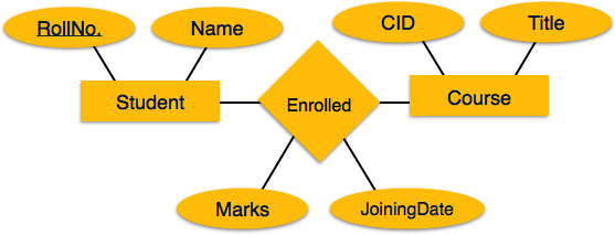
ER Model, when conceptualized into diagrams, gives a good overview of entity-relationship, which is easier to understand. ER diagrams can be mapped to relational schema, that is, it is possible to create relational schema using ER diagram. We cannot import all the ER constraints into relational model, but an approximate schema can be generated.

There are several processes and algorithms available to convert ER Diagrams into Relational Schema. Some of them are automated and some of them are manual. We may focus here on the mapping diagram contents to relational basics.

ER diagrams mainly comprise of −

• Entity and its attributes
• Relationship, which is association among entities.

Mapping Entity

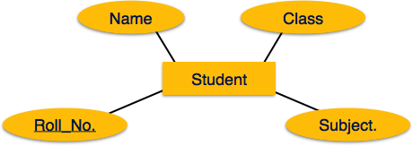
An entity is a real-world object with some attributes.

Mapping Process (Algorithm)

• Create table for each entity.
• Entity’s attributes should become fields of tables with their respective data types.
• Declare primary key.

Mapping Relationship

A relationship is an association among entities.

Mapping Process

• Create table for a relationship.
• Add the primary keys of all participating Entities as fields of table with their respective data types.
• If relationship has any attribute, add each attribute as field of table.
• Declare a primary key composing all the primary keys of participating entities.
• Declare all foreign key constraints.

Mapping Weak Entity Sets

A weak entity set is one which does not have any primary key associated with it.

Mapping Process

• Create table for weak entity set.
• Add all its attributes to table as field.
• Add the primary key of identifying entity set.
• Declare all foreign key constraints.

Mapping Hierarchical Entities

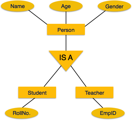
ER specialization or generalization comes in the form of hierarchical entity sets.

Mapping Process

• Create tables for all higher-level entities.
• Create tables for lower-level entities.
• Add primary keys of higher-level entities in the table of lower-level entities.
• In lower-level tables, add all other attributes of lower-level entities.
• Declare primary key of higher-level table and the primary key for lower-level table.
• Declare foreign key constraints.

In relational algebra, several operators are essential due to their unique functionalities. One such operator is the division operator, symbolized by “÷“. This operator is relatively complex but plays a crucial role in solving queries that involve the “all” condition. While many relational algebra operations focus on combining or filtering data, the division operation identifies tuples in one relation that are associated with every tuple in another.

In this chapter, we’ll explore the concept of the division operator in detail, understand its theoretical foundation, and walk through practical examples to grasp its application.

Basics of the Division Operator

The division operation applies to two relations −

• Numerator Relation (R) − Represents the main dataset and contains the superset of possible combinations.
• Denominator Relation (S) − Represents the subset or the set of conditions that must be satisfied.

The result is a relation containing only those tuples from the numerator that are associated with every tuple in the denominator.

Attributes in Relations

Let’s define the attributes involved in the division operator −

• R(Z) is the numerator, where Z = X ∪ Y
• S(X) is the denominator
• T(Y) is the result

Here, T contains the attributes in R that are not in S. For a tuple to appear in T, it must pair with every tuple in S within R.

To better understand the concept, consider a real-world scenario. Suppose we are organizing a workshop. Participants (R) are linked to sessions (X). We want to find those participants who attended all required sessions (S). The division operator helps identify these individuals by evaluating the “all sessions attended” condition.

Step-by-Step Explanation of the Division Operator

The division operation ensures that each result tuple in T(Y) must appear in R(Z) in combination with every tuple in S(X). Any tuple in R that fails to match all tuples in S is excluded from the result.

Mathematical Representation

The division operator can be expressed using a combination of projection, Cartesian product, and difference −

• T1 − Identify all potential result tuples: T1 ← π_Y(R)
• T2 − Find tuples in T1 that do not satisfy the pairing condition with S: T2 ← π_Y((S × T1) − R)
• Final Result − Subtract the unsatisfying tuples from the potential results. T ← T1 − T2

Example: Employees Working on All Projects

Let us take an example to get a clear understanding of how the division operator works.

Query − Find the names of employees who work on all projects that “John Smith” works on.

Relations Involved − Following are the relations involved in this query –

WORKS_ON − Contains tuples of employee IDs (Essn) and project numbers (Pno).

Essn	Pno	Hours
123456789	1	32.5
123456789	2	7.5
666884444	3	40.0
453453453	1	20.0
453453453	2	20.0
333445555	2	10.0
333445555	3	10.0
333445555	10	10.0
333445555	20	10.0
999887777	30	30.0
999887777	10	10.0
987987987	10	35.0
987987987	30	5.0
987654321	30	20.0
987654321	20	15.0
888665555	20	NULL

EMPLOYEE − Contains personal details like Fname, Lname, and Ssn.

Fname	Minit	Lname	Ssn	Bdate	Address	Sex	Salary	Super_ssn	Dno
John	B	Smith	123456789	1965-01-09	731 Fondren, Houston, TX	M	30000	333445555	5
Franklin	T	Wong	333445555	1955-12-08	638 Voss, Houston, TX	M	40000	888665555	5
Alicia	J	Zelaya	999887777	1968-01-19	3321 Castle, Spring, TX	F	25000	987654321	4
Jennifer	S	Wallace	987654321	1941-06-20	291 Berry, Bellaire, TX	F	43000	888665555	4
Ramesh	K	Narayan	666884444	1962-09-15	975 Fire Oak, Humble, TX	M	38000	333445555	5
Joyce	A	English	453453453	1972-07-31	5631 Rice, Houston, TX	F	25000	333445555	5
Ahmad	V	Jabbar	987987987	1969-03-29	980 Dallas, Houston, TX	M	25000	987654321	4
James	E	Borg	888665555	1937-11-10	450 Stone, Houston, TX	M	55000	NULL	1

Now, let’s understand step-by-step how to find the names of employees who work on all projects that “John Smith” works on.

Retrieve John Smith’s Projects

Start by filtering the projects linked to “John Smith.”

SMITH←σFname=′John′ANDLname=′Smith′(EMPLOYEE)

Fname	Minit	Lname	Ssn	Bdate	Address	Sex	Salary	Super_ssn	Dno
John	B	Smith	123456789	1965-01-09	731 Fondren, Houston, TX	M	30000	333445555	5

SMITHPNOS←πPno(WORKSON⋈Essn=SsnSMITH)

Pno
1
2

This gives a relation SMITH_PNOS containing all project numbers “John Smith” is assigned to.

Create All Employee-Project Relationships

Extract a relation showing all employees and their associated projects.

SSNPNOS←πEssn,Pno(WORKSON)

Essn	Pno
123456789	1
123456789	2
666884444	3
453453453	1
453453453	2
333445555	2
333445555	3
333445555	10
333445555	20
999887777	30
999887777	10
987987987	10
987987987	30
987654321	30
987654321	20
888665555	20

Apply Division

Use the division operator to find employees whose project assignments cover all projects in SMITH_PNOS.

SSNS(Ssn)←SSNPNOS÷SMITHPNOS

Ssn
123456789
453453453

Map Employee IDs to Names

Finally, retrieve the names of these employees.

RESULT←πFname,Lname(SSNS⋈EMPLOYEE)

Fname	Lname
John	Smith
Joyce	English

Final output − The final relation contains the names of employees who work on all the projects that “John Smith” works on.

Generalized Example: Products and Suppliers

Scenario − A store sells products (R) supplied by various suppliers (S). We want to identify products available from all suppliers.

Input Relations

• R − Contains ProductID and SupplierID
• S − Contains just SupplierID

Let’s go through its steps.

Extract potential products −

T1←πProductID(R)

Identify mismatched products −

T2←πProductID((S×T1)−R)

Subtract mismatches from potential products −

T←T1−T2

Output − If only certain products are supplied by every supplier, those product IDs will appear in the result relation T.

Key Observations

• Handling Universal Quantification − The division operator is useful for queries that require “for all” conditions. This is like finding students enrolled in all mandatory courses or employees assigned to every project in a list.
• Limitations in SQL − SQL does not directly support the division operator. However, similar results can be achieved using NOT EXISTS or complex joins. Although these approaches may lack the power of relational algebra.
• Practical Relevance − While it is theoretically significant, division is less common in practical database management systems due to its complexity and rare use cases.

Additional Applications

• Matching Preferences − Find customers whose preferences match every feature of a product.
• Cross-Department Participation − Identify employees involved in activities across all departments.

We understand the benefits of taking a Cartesian product of two relations, which gives us all the possible tuples that are paired together. But it might not be feasible for us in certain cases to take a Cartesian product where we encounter huge relations with thousands of tuples having a considerable large number of attributes.

Join is a combination of a Cartesian product followed by a selection process. A Join operation pairs two tuples from different relations, if and only if a given join condition is satisfied.

We will briefly describe various join types in the following sections.

Theta (θ) Join

Theta join combines tuples from different relations provided they satisfy the theta condition. The join condition is denoted by the symbol θ.

Notation

R1 ⋈θ R2

R1 and R2 are relations having attributes (A1, A2, .., An) and (B1, B2,.. ,Bn) such that the attributes dont have anything in common, that is R1 ∩ R2 = Φ.

Theta join can use all kinds of comparison operators.

Student
SID	Name	Std
101	Alex	10
102	Maria	11

Subjects
Class	Subject
10	Math
10	English
11	Music
11	Sports

Student_Detail −

STUDENT ⋈Student.Std = Subject.Class SUBJECT

Student_detail
SID	Name	Std	Class	Subject
101	Alex	10	10	Math
101	Alex	10	10	English
102	Maria	11	11	Music
102	Maria	11	11	Sports

Equijoin

When Theta join uses only equality comparison operator, it is said to be equijoin. The above example corresponds to equijoin.

Natural Join (⋈)

Natural join does not use any comparison operator. It does not concatenate the way a Cartesian product does. We can perform a Natural Join only if there is at least one common attribute that exists between two relations. In addition, the attributes must have the same name and domain.

Natural join acts on those matching attributes where the values of attributes in both the relations are same.

Courses
CID	Course	Dept
CS01	Database	CS
ME01	Mechanics	ME
EE01	Electronics	EE

HoD
Dept	Head
CS	Alex
ME	Maya
EE	Mira

Courses ⋈ HoD
Dept	CID	Course	Head
CS	CS01	Database	Alex
ME	ME01	Mechanics	Maya
EE	EE01	Electronics	Mira

Outer Joins

Theta Join, Equijoin, and Natural Join are called inner joins. An inner join includes only those tuples with matching attributes and the rest are discarded in the resulting relation. Therefore, we need to use outer joins to include all the tuples from the participating relations in the resulting relation. There are three kinds of outer joins − left outer join, right outer join, and full outer join.

Left Outer Join(R  S)

All the tuples from the Left relation, R, are included in the resulting relation. If there are tuples in R without any matching tuple in the Right relation S, then the S-attributes of the resulting relation are made NULL.

Left
A	B
100	Database
101	Mechanics
102	Electronics

Right
A	B
100	Alex
102	Maya
104	Mira

Courses  HoD
A	B	C	D
100	Database	100	Alex
101	Mechanics	—	—
102	Electronics	102	Maya

Right Outer Join: ( R  S )

All the tuples from the Right relation, S, are included in the resulting relation. If there are tuples in S without any matching tuple in R, then the R-attributes of resulting relation are made NULL.

Courses  HoD
A	B	C	D
100	Database	100	Alex
102	Electronics	102	Maya
—	—	104	Mira

Full Outer Join: ( R  S)

All the tuples from both participating relations are included in the resulting relation. If there are no matching tuples for both relations, their respective unmatched attributes are made NULL.

Courses  HoD
A	B	C	D
100	Database	100	Alex
101	Mechanics	—	—
102	Electronics	102	Maya
—	—	104	Mira

In relational algebra we use several set theory operations. Since relational model is based on set theory it borrows several concepts from set theory as well in respect to the operations. These include UNION, INTERSECTION, MINUS (also called SET DIFFERENCE), and also the CARTESIAN PRODUCT. In this article, we will see down each operator and work through examples for a better understanding.

Let us see the following two tables that we will focus in the next examples −

In relational algebra, several operations are derived from set theory. Since the relational model is based on set theory, it adopts key concepts such as UNION, INTERSECTION, MINUS (also called SET DIFFERENCE), and CARTESIAN PRODUCT.

In this chapter, we will examine each of these operators with practical examples for better understanding. Let’s begin by reviewing two tables that will be used in the upcoming examples −

EMPLOYEE Table

Fname	Minit	Lname	Ssn	Bdate	Address	Sex	Salary	Super_ssn	Dno
John	B	Smith	123456789	1965-01-09	731 Fondren, Houston, TX	M	30000	333445555	5
Franklin	T	Wong	333445555	1955-12-08	638 Voss, Houston, TX	M	40000	888665555	5
Alicia	J	Zelaya	999887777	1968-01-19	3321 Castle, Spring, TX	F	25000	987654321	4
Jennifer	S	Wallace	987654321	1941-06-20	291 Berry, Bellaire, TX	F	43000	888665555	4
Ramesh	K	Narayan	666884444	1962-09-15	975 Fire Oak, Humble, TX	M	38000	333445555	5
Joyce	A	English	453453453	1972-07-31	5631 Rice, Houston, TX	F	25000	333445555	5
Ahmad	V	Jabbar	987987987	1969-03-29	980 Dallas, Houston, TX	M	25000	987654321	4
James	E	Borg	888665555	1937-11-10	450 Stone, Houston, TX	M	55000	NULL	1

DEPENDENT Table

Essn	Dependent_name	Sex	Bdate	Relationship
333445555	Alice	F	1986-04-05	Daughter
333445555	Theodore	M	1983-10-25	Son
333445555	Joy	F	1958-05-03	Spouse
987654321	Abner	M	1942-02-28	Spouse
123456789	Michael	M	1988-01-04	Son
123456789	Alice	F	1988-12-30	Daughter
123456789	Elizabeth	F	1967-05-05	Spouse

Set Theory Basics in Relational Algebra

In set theory, each element in a set is unique, and operations like UNION and INTERSECTION combine or compare these elements systematically. Relational algebra applies similar principles by treating each row in a table as a set element.

However, relational tables have more structure than simple sets, so additional rules apply −

• Union Compatibility − For operations like UNION and INTERSECTION, the tables must have the same number of attributes, and each attribute must have the same data type.
• Duplicate Elimination − These operations inherently remove duplicates, as relational algebra operates on sets, not multisets.

The UNION Operator

The UNION operator combines rows from two relations, producing a result with all unique rows present in either relation-similar to merging two lists while removing duplicates.

Syntax and Representation

In relational algebra, UNION is represented as −

R ∪ S

Here, R and S are two relations (tables) that must be union compatible.

Combining Employee and Manager IDs

Let us consider we want a find of all employees who either work in department 5 or supervise someone in department 5. We use UNION to merge these groups −

Retrieve Social Security numbers (SSN) of employees in department 5 −

RESULT1 ← πSsn(σDno =5(EMPLOYEE))

Ssn
123456789
333445555
666884444
453453453

Retrieve SSNs of managers supervising department 5 employees −

RESULT2 ← πSuper_ssn(σDno =5(EMPLOYEE))

Super_ssn
333445555
888665555
333445555
333445555

Combine both lists −

RESULT ← RESULT1 ∪ RESULT2

Ssn
123456789
333445555
666884444
453453453
333445555
888665555
333445555
333445555

The final table will include SSNs of all employees who meet either condition. For instance, if RESULT1 contains {123, 456} and RESULT2 contains {456, 789}, the UNION result is {123, 456, 789}.

The INTERSECTION Operator

The INTERSECTION operator identifies rows present in both relations. It is like finding the overlap between two groups.

Syntax and Representation

INTERSECTION is denoted as −

R ∩ S

Finding SSN which are common in manager and employee

Consider the table of SSN of employees who work for department 1 and 5 −

RESULT1 ← πSsn(σDno =5^ Dno =1(EMPLOYEE))

Ssn
123456789
333445555
666884444
453453453
888665555

Retrieve SSNs of managers supervising department 5 employees −

RESULT2 ← πSuper_ssn(σDno =5(EMPLOYEE))

Super_ssn
333445555
888665555
333445555
333445555

The common SSN values are −

RESULT ← RESULT1 ∩ RESULT2

Ssn
333445555
888665555

The MINUS (SET DIFFERENCE) Operator

The MINUS operator, also called SET DIFFERENCE, is used to remove rows in one relation that appear in another. It essentially answers the question, “What is in one table but not the other?”

Syntax and Representation

In relational algebra, MINUS is represented as −

R − S

SSN of employees who are not manager

Consider the table of SSN of employees who work for department 1 and 5 −

RESULT1 ← πSsn(σDno =5^ Dno =1(EMPLOYEE))

Ssn
123456789
333445555
666884444
453453453
888665555

Retrieve SSNs of managers supervising department 5 employees −

RESULT2 ← πSuper_ssn(σDno =5(EMPLOYEE))

Super_ssn
333445555
888665555
333445555
333445555

The SSN of non-managers are −

RESULT ← RESULT1 − RESULT2

Ssn
123456789
666884444
453453453

The CARTESIAN PRODUCT (CROSS PRODUCT) Operator

The CARTESIAN PRODUCT operator combines every row of one table with every row of another. This operation produces all possible combinations of rows between the two tables. This can result in a large and often unwieldy table.

Syntax and Representation

In relational algebra, CARTESIAN PRODUCT is represented as −

R × S

Combining Employees with Dependents

Suppose we have a table EMPLOYEE and another table DEPENDENT. To pair every employee with every dependent −

EMP_DEPENDENTS ← EMPLOYEE × DEPENDENT

The resulting table will include every possible combination of rows from EMPLOYEE and DEPENDENT. However, this raw result is rarely useful on its own. Usually, we filter the combined rows using a SELECT operation to create meaningful connections.

Fname	Lname	Ssn	Essn	Dependent_name	Sex	Bdate	…
Alicia	Zelaya	999887777	333445555	Alice	F	1986-04-05	…
Alicia	Zelaya	999887777	333445555	Theodore	M	1983-10-25	…
Alicia	Zelaya	999887777	333445555	Joy	F	1958-05-03	…
Alicia	Zelaya	999887777	987654321	Abner	M	1942-02-28	…
Alicia	Zelaya	999887777	123456789	Michael	M	1988-01-04	…
Alicia	Zelaya	999887777	123456789	Alice	F	1988-12-30	…
Alicia	Zelaya	999887777	123456789	Elizabeth	F	1967-05-05	…
Jennifer	Wallace	987654321	333445555	Alice	F	1986-04-05	…
Jennifer	Wallace	987654321	333445555	Theodore	M	1983-10-25	…
Jennifer	Wallace	987654321	333445555	Joy	F	1958-05-03	…
Jennifer	Wallace	987654321	987654321	Abner	M	1942-02-28	…
Jennifer	Wallace	987654321	123456789	Michael	M	1988-01-04	…
Jennifer	Wallace	987654321	123456789	Alice	F	1988-12-30	…
Jennifer	Wallace	987654321	123456789	Elizabeth	F	1967-05-05	…
Joyce	English	453453453	333445555	Alice	F	1986-04-05	…
Joyce	English	453453453	333445555	Theodore	M	1983-10-25	…
Joyce	English	453453453	333445555	Joy	F	1958-05-03	…
Joyce	English	453453453	987654321	Abner	M	1942-02-28	…
Joyce	English	453453453	123456789	Michael	M	1988-01-04	…
Joyce	English	453453453	123456789	Alice	F	1988-12-30	…
Joyce	English	453453453	123456789	Elizabeth	F	1967-05-05	…

The table is truncated for space otherwise it will be much larger.

Sequences and Combined Operations

Relational algebra becomes useful when we combine operators. Sometimes, the result of one operation feeds into another. This is allowing us to answer complex queries.

Female Employees and Their Dependents

To find dependents of female employees −

Filter female employees −

FEMALE_EMPS ← σSex=′F′(EMPLOYEE)

Retrieve names and SSNs of female employees −

EMP_NAMES ← πFname,Lname,Ssn(FEMALE_EMPS)

Combine with the DEPENDENT table −

EMP_DEPENDENTS ← EMP_NAMES × DEPENDENT

Match dependents to employees by SSN −

ACTUAL_DEPENDENTS ← σSsn=Essn(EMP_DEPENDENTS)

Extract names of employees and their dependents −

πFname,Lname,Dependent_name(ACTUAL_DEPENDENTS)

This sequence demonstrates how CARTESIAN PRODUCT and SELECT work together to filter meaningful relationships from raw combinations.

SQL Equivalents of Set Theory Operators

These relational operators have direct counterparts in SQL −

• UNION − Combines results from two queries, removing duplicates unless UNION ALL is used.
• INTERSECT − Retrieves rows common to both queries.
• EXCEPT (or MINUS) − Retrieves rows in one query but not the other.
• CROSS JOIN − Implements CARTESIAN PRODUCT in SQL.

Example in SQL

For the UNION operation −

SELECT Ssn
FROM EMPLOYEE
WHERE Dno =5UNIONSELECT Super_ssn
FROM EMPLOYEE
WHERE Dno =5;

The relational model plays a key role in organizing and managing data. At its core lies relational algebra, a set of operations that enables users to efficiently manipulate and query data. Among these are unary operations such as SELECT and PROJECT, which are essential tools for filtering and organizing data.

In this chapter, we will explore these two unary relational operations (SELECT and PROJECT), understand how they work, and provide examples to make it easier for you to understand.

In all the examples throughout this chapter, we will use the following Sample Data Table called EMPLOYEE:

Fname	Minit	Lname	Ssn	Bdate	Address	Sex	Salary	Super_ssn	Dno
John	B	Smith	123456789	1965-01-09	731 Fondren, Houston, TX	M	30000	333445555	5
Franklin	T	Wong	333445555	1955-12-08	638 Voss, Houston, TX	M	40000	888665555	5
Alicia	J	Zelaya	999887777	1968-01-19	3321 Castle, Spring, TX	F	25000	987654321	4
Jennifer	S	Wallace	987654321	1941-06-20	291 Berry, Bellaire, TX	F	43000	888665555	4
Ramesh	K	Narayan	666884444	1962-09-15	975 Fire Oak, Humble, TX	M	38000	333445555	5
Joyce	A	English	453453453	1972-07-31	5631 Rice, Houston, TX	F	25000	333445555	5
Ahmad	V	Jabbar	987987987	1969-03-29	980 Dallas, Houston, TX	M	25000	987654321	4
James	E	Borg	888665555	1937-11-10	450 Stone, Houston, TX	M	55000	NULL	1

Understanding the SELECT Operation

The SELECT operation allows us to retrieve a subset of rows (or tuples) from a table (or relation) that satisfy a specific condition. It acts like a filter. It is keeping only the rows that meet the specified criteria while discarding the rest. The resulting table keeps all the original attributes of the filtered rows.

Syntax and Representation

In relational algebra, the representation of SELECT operation is very simple:

σcondition(R)

Here:

• σ (sigma): Symbolizes the SELECT operation
• condition: Specifies the criteria to filter the rows
• R: Name of the relation or table being operated upon

Example: Filtering by Department Number

Suppose we have a table named EMPLOYEE with attributes such as department number (Dno) and salary.

To retrieve the rows for employees in department 4, we write:

σDno=4(EMPLOYEE)

It will fetch the following records –

Fname	Minit	Lname	Ssn	Bdate	Address	Sex	Salary	Super_ssn	Dno
Alicia	J	Zelaya	999887777	1968-01-19	3321 Castle, Spring, TX	F	25000	987654321	4
Jennifer	S	Wallace	987654321	1941-06-20	291 Berry, Bellaire, TX	F	43000	888665555	4
Ahmad	V	Jabbar	987987987	1969-03-29	980 Dallas, Houston, TX	M	25000	987654321	4

Example: Filtering by Salary

To retrieve employees earning more than $30,000, we can write the query as follows:

σSalary>30000(EMPLOYEE)

It will fetch the following records –

Fname	Minit	Lname	Ssn	Bdate	Address	Sex	Salary	Super_ssn	Dno
Franklin	T	Wong	333445555	1955-12-08	638 Voss, Houston, TX	M	40000	888665555	5
Jennifer	S	Wallace	987654321	1941-06-20	291 Berry, Bellaire, TX	F	43000	888665555	4
Ramesh	K	Narayan	666884444	1962-09-15	975 Fire Oak, Humble, TX	M	38000	333445555	5
James	E	Borg	888665555	1937-11-10	450 Stone, Houston, TX	M	55000	NULL	1

Combining Multiple Conditions

The SELECT operation supports combining multiple conditions using Boolean operators like AND, OR, and NOT.

Example: Complex Filtering

Let us see another example where we merge multiple conditions. To find employees working in department 4 with a salary above 25,000orindepartment5withasalaryabove30,000, we can write the following complex query:

σ(Dno=4∧Salary>25000)∨(Dno=5∧Salary>30000)(EMPLOYEE)

It will fetch the following records –

Fname	Minit	Lname	Ssn	Bdate	Address	Sex	Salary	Super_ssn	Dno
Franklin	T	Wong	333445555	1955-12-08	638 Voss, Houston, TX	M	40000	888665555	5
Jennifer	S	Wallace	987654321	1941-06-20	291 Berry, Bellaire, TX	F	43000	888665555	4
Ramesh	K	Narayan	666884444	1962-09-15	975 Fire Oak, Humble, TX	M	38000	333445555	5

This operation results in a filtered table with only those rows that satisfy at least one of the conditions.

From the corresponding examples, one thing we understood that the SELECT operation is commutative, which means,

σcond1(σcond2(R))=σcond2(σcond1(R))

SELECT does not alter the structure of the table; only the number of rows changes.

Understanding the PROJECT Operation

The PROJECT operation targets columns. It creates a new table with only the specified attributes, discarding all others. This operation is useful when we need to focus on specific fields from a dataset.

Syntax and Representation

In relational algebra, the PROJECT operation can be denoted as:

πattribute_list(R)

Here:

• π (pi): symbolizes the PROJECT operation.
• attribute_list: specifies the columns to include in the result.
• R is the relation being projected.

Example: Retrieving Specific Attributes

Let us see some examples from simpler to complex. If we want to list only the first name, last name, and salary of employees from the EMPLOYEE table, we write the query in the following format.

πFname,Lname,Salary(EMPLOYEE)

The resulting table will contain only the selected columns –

Fname	Lname	Salary
John	Smith	30000
Franklin	Wong	40000
Alicia	Zelaya	25000
Jennifer	Wallace	43000
Ramesh	Narayan	38000
Joyce	English	25000
Ahmad	Jabbar	25000
James	Borg	55000

Duplicate Elimination in PROJECT

A critical aspect of PROJECT is that it eliminates duplicate rows. If two rows in the original table have the same values for the projected columns, only one will appear in the result.

Example: Duplicate Elimination

To list unique combinations of gender (Sex) and salary, use:

πSex,Salary(EMPLOYEE)

This gives that any duplicate rows in the Sex and Salary columns are removed in the output.

Sex	Salary
M	30000
M	40000
F	25000
F	43000
M	38000
M	25000
M	55000

“F 25000” is removed since it is duplicate.

Sequences and Naming in Operations

For more complex queries, we often combine SELECT and PROJECT operations. These sequences can either be written as nested expressions or broken down into steps with intermediate results.

Example: Combining SELECT and PROJECT

To find the first name, last name, and salary of employees in department 5, we can write:

First, apply the SELECT operation:

TEMP⟵σDno=5(EMPLOYEE)

It will fetch the following records –

Fname	Minit	Lname	Ssn	Bdate	Address	Sex	Salary	Super_ssn	Dno
John	B	Smith	123456789	1965-01-09	731 Fondren, Houston, TX	M	30000	333445555	5
Franklin	T	Wong	333445555	1955-12-08	638 Voss, Houston, TX	M	40000	888665555	5
Ramesh	K	Narayan	666884444	1962-09-15	975 Fire Oak, Humble, TX	M	38000	333445555	5
Joyce	A	English	453453453	1972-07-31	5631 Rice, Houston, TX	F	25000	333445555	5

Next, apply the PROJECT operation:

RESULT⟵πFname,Lname,Salary(TEMP)

It will fetch the following records –

Fname	Lname	Salary
John	Smith	30000
Franklin	Wong	40000
Ramesh	Narayan	38000
Joyce	English	25000

Alternatively, this can be combined into a single inline expression:

πFname,Lname,Salary(σDno=5(EMPLOYEE))

Renaming the Attributes

Sometimes, the resulting table from a sequence of operations needs attribute names to be changed for clarity. The RENAME operation, denoted by “ρ” (rho), allows us to rename the attributes or the table itself.

For example:

ρ(First_Name, Last_Name, Salary)⟵πFname,Lname,Salary(EMPLOYEE)

Applications of SELECT and PROJECT Operations in SQL

In SQL, the SELECT and PROJECT operations are mirrored in the SELECT clause and the WHERE clause of a query. For example:

The relational algebra expression “σDno=4∧Salary>25000(EMPLOYEE)” corresponds to:

SELECT*FROM EMPLOYEE 
WHERE Dno =4AND Salary >25000;

The PROJECT operation “πSex,Salary(EMPLOYEE)” translates to:

SELECTDISTINCT Sex, Salary 
FROM EMPLOYEE;

Relational database systems are expected to be equipped with a query language that can assist its users to query the database instances. There are two kinds of query languages − relational algebra and relational calculus.

Relational Algebra

Relational algebra is a procedural query language, which takes instances of relations as input and yields instances of relations as output. It uses operators to perform queries. An operator can be either unary or binary. They accept relations as their input and yield relations as their output. Relational algebra is performed recursively on a relation and intermediate results are also considered relations.

The fundamental operations of relational algebra are as follows −

• Select
• Project
• Union
• Set different
• Cartesian product
• Rename

We will discuss all these operations in the following sections.

Select Operation (σ)

It selects tuples that satisfy the given predicate from a relation.

Notation − σ_p(r)

Where σ stands for selection predicate and r stands for relation. p is prepositional logic formula which may use connectors like and, or, and not. These terms may use relational operators like − =, ≠, ≥, < ,  >,  ≤.

For example −

σsubject = "database"(Books)

Output − Selects tuples from books where subject is ‘database’.

σsubject = "database" and price = "450"(Books)

Output − Selects tuples from books where subject is ‘database’ and ‘price’ is 450.

σsubject = "database" and price = "450" or year > "2010"(Books)

Output − Selects tuples from books where subject is ‘database’ and ‘price’ is 450 or those books published after 2010.

Project Operation (∏)

It projects column(s) that satisfy a given predicate.

Notation − ∏_{A1, A2, An} (r)

Where A₁, A₂ , A_n are attribute names of relation r.

Duplicate rows are automatically eliminated, as relation is a set.

For example −

∏subject, author (Books)

Selects and projects columns named as subject and author from the relation Books.

Union Operation (∪)

It performs binary union between two given relations and is defined as −

r ∪ s = { t | t ∈ r or t ∈ s}

Notation − r U s

Where r and s are either database relations or relation result set (temporary relation).

For a union operation to be valid, the following conditions must hold −

• r, and s must have the same number of attributes.
• Attribute domains must be compatible.
• Duplicate tuples are automatically eliminated.

∏ author (Books) ∪ ∏ author (Articles)

Output − Projects the names of the authors who have either written a book or an article or both.

Set Difference (−)

The result of set difference operation is tuples, which are present in one relation but are not in the second relation.

Notation − r − s

Finds all the tuples that are present in r but not in s.

∏ author (Books) − ∏ author (Articles)

Output − Provides the name of authors who have written books but not articles.

Cartesian Product (Χ)

Combines information of two different relations into one.

Notation − r Χ s

Where r and s are relations and their output will be defined as −

r Χ s = { q t | q ∈ r and t ∈ s}

σauthor = 'tutorialspoint'(Books Χ Articles)

Output − Yields a relation, which shows all the books and articles written by tutorialspoint.

Rename Operation (ρ)

The results of relational algebra are also relations but without any name. The rename operation allows us to rename the output relation. ‘rename’ operation is denoted with small Greek letter rho ρ.

Notation − ρ _x (E)

Where the result of expression E is saved with name of x.

Additional operations are −

• Set intersection
• Assignment
• Natural join

Relational Calculus

In contrast to Relational Algebra, Relational Calculus is a non-procedural query language, that is, it tells what to do but never explains how to do it.

Relational calculus exists in two forms −

Tuple Relational Calculus (TRC)

Filtering variable ranges over tuples

Notation − {T | Condition}

Returns all tuples T that satisfies a condition.

For example −

{ T.name |  Author(T) AND T.article = 'database' }

Output − Returns tuples with ‘name’ from Author who has written article on ‘database’.

TRC can be quantified. We can use Existential (∃) and Universal Quantifiers (∀).

For example −

{ R| ∃T   ∈ Authors(T.article='database' AND R.name=T.name)}

Output − The above query will yield the same result as the previous one.

Domain Relational Calculus (DRC)

In DRC, the filtering variable uses the domain of attributes instead of entire tuple values (as done in TRC, mentioned above).

Notation −

{ a₁, a₂, a₃, …, a_n | P (a₁, a₂, a₃, … ,a_n)}

Where a1, a2 are attributes and P stands for formulae built by inner attributes.

For example −

{ |  ∈ TutorialsPoint ∧ subject = 'database'}

Output − Yields Article, Page, and Subject from the relation TutorialsPoint, where subject is database.

Just like TRC, DRC can also be written using existential and universal quantifiers. DRC also involves relational operators.

The expression power of Tuple Relation Calculus and Domain Relation Calculus is equivalent to Relational Algebra.