Author: saqibkhan

  • Relational Database Schemas

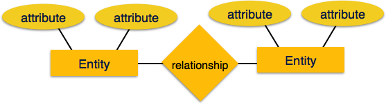
    In a relational database model, the structure of data is maintained through a defined schema. A relational schema serves as the framework that outlines how data is organized and managed within a relational database. It includes attributes and the relationships between them. This framework ensures that data is stored in a way that maintains consistency and integrity.

    In this chapter, we will explore relational database schemas in depth, understand key concepts through examples, and explain how constraints help maintain data reliability.

    Relational Database Schema

    A relational database schema, represented by S, acts as a map for how data is structured in the database. It consists of a set of relation schemas and a collection of integrity constraints.

    The schema outlines how data interacts within and between tables. Each relation schema specifies the table’s name, its attributes, and their domains.

    Components of a Schema

    A relational schema has three major components:

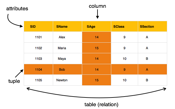
    • Relation Schema (R) − The structure of a table, written as R(A1, A2, …, An), where A1, A2, …, An are attributes.
    • Attribute − A column within a table, each with a specific domain that limits the type of data it can contain.
    • Database State (DB) − The current data held in all tables conforming to the schema. A valid state meets all schema constraints.

    Example − Consider a relational schema for a COMPANY database:

    • EMPLOYEE (Ssn, Name, Salary, Dno)
    • DEPARTMENT (Dnumber, Dname, Mgr_ssn, Mgr_start_date)
    • PROJECT (Pnumber, Pname, Plocation, Dnum)

    Each relation schema outlines the columns of its respective table. It also indicates how data should be represented.

    Relational Database Schemas – Key Features and Components

    Let us now understand some of the key features and components of Relational Database Schemas:

    Attributes and Their Domains

    Every attribute within a relation schema has an associated domain that defines its allowable values. The domains enforce data type restrictions and value limits, ensuring consistency within the database.

    Consider an example where the Ssn attribute in the EMPLOYEE table might be limited to a pattern that matches valid social security numbers (e.g., XXX-XX-XXXX). Similarly the Age attribute could be restricted to integer values between 18 and 65.

    We know domains help prevent errors by ensuring the supplied data conforms to expected types and formats. So, an Age attribute defined with INTEGER CHECK (Age BETWEEN 18 AND 65) would block an insertion of Age = 17 or Age = 70.

    Relation States

    relation state is the set of tuples (rows) that exist in a table at any given time. Each tuple must comply with the attribute domains defined in the schema.

    For a better understanding, consider the following EMPLOYEE table with data:

    FnameLnameSsnSalaryDno
    JohnSmith123456789300005
    FranklinWong333445555400005
    AliciaZelaya999887777250004
    JenniferWallace987654321430004
    RameshNarayan666884444380005
    JoyceEnglish453453453250005
    AhmadJabbar987987987250004
    JamesBorg888665555550001

    For example, a tuple in the EMPLOYEE table might be represented as,

    <John, Smith,123-45-6789,30000,5>

    This tuple states that John Smith, identified by his Ssn, earns a salary of $30,000 and works in the department with Dno = 5. (We have removed other attributes for simplicity)

    Integrity Constraints

    Integrity constraints make sure that the data remains accurate and logically consistent. Integrity constraints include:

    • Key Constraints − Enforce uniqueness for specified attributes, known as keys, so that no two tuples share the same values for these attributes.
    • Entity Integrity − Ensures primary key attributes cannot have NULL values, maintaining the uniqueness and identifiability of each tuple.
    • Referential Integrity − Ensures foreign keys match primary keys in related tables or are NULL.
    DnameDnumberMgr_ssnMgr_start_date
    Research53334455551988-05-22
    Administration49876543211995-01-01
    Headquarters18886655551981-06-19

    In the COMPANY database, the Dno attribute in the EMPLOYEE table is a foreign key referencing the Dnumber attribute in the DEPARTMENT table. If an EMPLOYEE record has Dno = 5, Dnumber = 5 must exist in the DEPARTMENT table for referential integrity to hold.

    Practical Examples of Relational Database Schemas

    Let us go through the COMPANY database schema and see how the tables relate and enforce constraints.

    Here is the PROJECT table:

    PnamePnumberPlocationDnum
    ProductX1Bellaire5
    ProductY2Sugarland5
    ProductZ3Houston5
    Computerization10Stafford4
    Reorganization20Houston1
    Newbenefits30Stafford4
    • EMPLOYEE (Ssn, Name, Salary, Dno) − The Ssn attribute acts as the primary key, uniquely identifying each employee. The Dno attribute is a foreign key referencing Dnumber in the DEPARTMENT table.
    • DEPARTMENT (Dnumber, Dname, Mgr_ssn, Mgr_start_date) − The Dnumber attribute is the primary key, uniquely identifying each department. The Mgr_ssn attribute references Ssn in the EMPLOYEE table, indicating which employee manages the department.
    • PROJECT (Pnumber, Pname, Plocation, Dnum) − Pnumber serves as the primary key. Dnum is a foreign key referencing Dnumber in DEPARTMENT.

    If an employee record is inserted with Dno = 10, but Dnumber = 10 does not exist in the DEPARTMENT table, the insertion will be rejected due to a referential integrity violation.

    Super Keys and Candidate Keys

    Super keys and candidate keys help identify unique tuples within a relation.

    • The term “super key” is used for any combination of attributes that uniquely identifies a tuple.
    • A candidate key is a minimal super key without redundant attributes.

    Consider a CAR schema:

    CAR (License_number, Engine_serial_number, Make, Model)

    In this case,

    • License_number is a candidate key, as it uniquely identifies each car.
    • License_number, Engine_serial_number together is a superkey, but not minimal, so it is not a candidate key.

    The Importance of Primary Keys

    A primary key is nothing but a chosen candidate key. It must have unique, non-NULL values. This constraint ensures every record can be uniquely identified.

    For example, Ssn is the primary key in the EMPLOYEE table. Trying to insert a record with Ssn = NULL will violate entity integrity, resulting in a rejected insertion.

    Relationships and Foreign Keys

    Foreign keys are attributes in one table that link to primary keys in another. Foreign keys are meant for creating relationship between tables. They help ensure consistency when dealing with related data.

    Consider the WORKS_ON table with attributes Essn and Pno:

    EssnPnoHours
    123456789132.5
    12345678927.5
    666884444340.0
    453453453120.0
    453453453220.0
    333445555210.0
    333445555310.0
    3334455551010.0
    3334455552010.0
    9998877773030.0
    9998877771010.0
    9879879871035.0
    987987987305.0
    9876543213020.0
    9876543212015.0
    88866555520NULL

    Essn references Ssn in EMPLOYEE, and Pno references Pnumber in PROJECT. This relationship defines which employees are working on which projects.

    Violation Case − If an employee’s Ssn is deleted from EMPLOYEE but still exists as Essn in WORKS_ON, then referential integrity gets violated unless action is taken (e.g., cascading the delete or setting Essn to NULL).

    Conclusion

    To conclude, relational database schemas are foundational for defining how data is structured and managed. In this chapter, we highlighted the components of a schema, such as relation schemas, attributes, and their domains. Thereafter, we used the COMPANY schema to illustrate the importance of primary and foreign keys. We also understood how integrity constraints like entity and referential integrity help maintain data reliability.

  • Relational Model Constraints

    Relational databases are widely used; they provide structured and reliable ways to store and access the data. To ensure data integrity and consistency, relational databases mostly rely on certain rules known as constraints. These constraints are used to maintain the quality and reliability of data across different tables and records.

    In this chapter, we will take a look at the types of relational model constraints, supplemented with practical examples and explanations for a better understanding.

    Relational Model Constraints

    Relational model constraints are set of rules applied to the structure and data of a database to maintain logical consistency. They ensure that data is valid according to the rules defined in the database schema. These constraints can be broken down into three main types as given below −

    • Inherent model-based constraints − Implied by the nature of the relational model itself.
    • Schema-based constraints − Explicitly defined within the database schema and enforced by the database system.
    • Application-based constraints − Managed through external application logic as they cannot be directly expressed in the schema.

    Types of Relational Model Constraints

    Relational model constraints can be of the following types −

    • Domain Constraints
    • Key Constraints
    • Entity Integrity Constraint
    • Referential Integrity Constraint

    Let’s understand each of these in detail.

    Domain Constraints

    Domain constraints are used to specify that, every attribute in a database must contain only values from a predefined set known as domain. This ensures that each column in a table holds data of a particular type and format.

    For example, consider an EMPLOYEE table with an Age column that only allows integer values between 18 and 65. This domain constraint ensures that inserting a value such as “17” or “70” would violate the rule and be rejected by the system.

    If we define Age as INTEGER CHECK (Age BETWEEN 18 AND 65), any attempt to insert Age = 17 will trigger an error. The domain constraints is used to maintain data accuracy by preventing improper data types or out-of-bounds values.

    Key Constraints

    Key constraints are used for each record within a relation. It can be uniquely identified. This uniqueness is achieved through keys.

    Keys can be of the following types −

    • Superkey − Any set of attributes that uniquely identifies a tuple in a relation.
    • Candidate key − A minimal superkey. Removing any attribute would break the uniqueness property.
    • Primary key − A chosen candidate key that uniquely identifies each tuple in the table.

    For example, consider a table called STUDENT as given below −

    NameSSNHome PhoneAddressOffice PhoneAgeGPA
    Dick Davidson422-11-2320NULL3452 Elgin Road(817)749-1253253.53
    Barbara Benson533-69-1238(817)839-84617384 Fontana LaneNULL193.25
    Rohan Panchal489-22-1100(817)376-9821265 Lark Lane(817)749-6492283.93
    Chung-cha Kim381-62-1245(817)375-4409125 Kirby RoadNULL182.89
    Benjamin Bayer305-61-2435(817)373-16162918 Bluebonnet LaneNULL193.21

    The SSN (Social Security Number) serves as a primary key because each student must have a unique SSN. The primary key constraint guarantees that no two students can have the same SSN.

    This is important because the primary keys help to maintain the identity of each record. If a STUDENT table did not have a primary key, then distinguishing between duplicate records would be difficult, which will lead to a potential data ambiguity.

    Entity Integrity Constraint

    The entity integrity constraint states that, the primary key of a relation must always have a non-NULL value. It is needed because primary keys are used to identify tuples, and a NULL value would make identification impossible.

    Consider a table called CUSTOMER. If Customer_ID is defined as the primary key, then any attempt to insert a record with “Customer_ID = NULL” will violet the entity integrity constraint. It will be rejected by the system.

    Practically, we can consider a situation where a banking system has a Customer relation with primary keys representing account numbers. If one record had Account_ID = NULL, then it would be impossible to reference or link this record.

    Referential Integrity Constraint

    Referential integrity constraint states that, the relationships between tables remain consistent. A foreign key in one table must either match a primary key value in another table or be NULL. This constraint can preserve the logical connections between records in different tables.

    Suppose we have an EMPLOYEE table with a Dno column. Here, it references the Dnumber from the DEPARTMENT table. If Dno is set to a value that does not exist in the DEPARTMENT table, then it violates the referential integrity constraint.

    Detailed Scenario − See the Employee table −

    FnameMinitLnameSSNBdateAddressSexSalarySuper_ssnDno
    JohnBSmith1234567891965-01-09731 Fondren, Houston, TXM300003334455555
    FranklinTWong3334455551955-12-08638 Voss, Houston, TXM400008886655555
    AliciaJZelaya9998877771968-01-193321 Castle, Spring, TXF250009876543214
    JenniferSWallace9876543211941-06-20291 Berry, Bellaire, TXF430008886655554
    RameshKNarayan6668844441962-09-15975 Fire Oak, Humble, TXM380003334455555
    JoyceAEnglish4534534531972-07-315631 Rice, Houston, TXF250003334455555
    AhmadVJabbar9879879871969-03-29980 Dallas, Houston, TXM250009876543214
    JamesEBorg8886655551937-11-10450 Stone, Houston, TXM55000NULL1

    See the Department table −

    DnameDnumberMgr_ssnMgr_start_date
    Research53334455551988-05-22
    Administration49876543211995-01-01
    Headquarters18886655551981-06-19

    Valid Insertion − Adding an EMPLOYEE with Dno = 4 is allowed if Dnumber = 4 exists in DEPARTMENT.

    Violation Example − Inserting an EMPLOYEE with Dno = 99, where Dnumber = 99 does not exist in DEPARTMENT, would be rejected.

    This constraint is particularly useful in maintaining relationships between parent and child tables. So, deleting a department referenced by employees must either be restricted or cascaded to maintain integrity.

    Handling Constraint Violations

    In this section, let’s understand the kind of operations that can cause constraint violations and what precautionary measures can be taken in order to prevent such operations.

    Insertion Violations

    An insertion operation can violate various constraints because of −

    • Domain Constraint Violation − Inserting a non-integer value in an Age column defined as an integer will be rejected.
    • Key Constraint Violation − Adding a tuple with a duplicate Ssn in a STUDENT table where Ssn is the primary key will result in an error.
    • Entity Integrity Violation − Attempting to insert a row with NULL as the primary key value violates the entity integrity constraint.
    • Referential Integrity Violation − Inserting an EMPLOYEE with a Dno value that does not match any Dnumber in DEPARTMENT.

    Deletion and Referential Integrity

    Deleting a tuple can trigger constraint violations, particularly for referential integrity. For example, deleting the DEPARTMENT record that is referenced by the Dno of an EMPLOYEE tuple results in referential integrity issues.

    We can solve this issue by Restrict operation, like prevent deletion if it causes a violation. Or cascade, that is, automatically delete all dependent records. There is another solution: Set NULL / Default, i.e., modify the foreign key in dependent records to NULL or a default value.

    Update Operations

    Updating a record can affect primary keys and foreign keys. Modifying a primary key is similar to deleting the original record and inserting a new one, which may violate existing constraints. Updates can be two types:

    • Safe Update − Changing an employee’s salary does not affect primary or foreign keys and is permissible.
    • Risky Update − Modifying Ssn in EMPLOYEE to an existing Ssn violates the primary key constraint.

    Other Constraints and Business Rules

    We have studied the rules, but there are some other application-based constraints, or business rules. These rules include those that cannot be easily defined within the schema, such as −

    • “An employee’s salary must not exceed that of their supervisor.”
    • “Total weekly working hours for an employee should not exceed 56 hours.”

    These are typically enforced using application logic or triggers.

    Conclusion

    In this chapter, we presented an elaborate explanation of how relational model constraints play a crucial role in maintaining data integrity and consistency in a database. We understood the different types of constraints, such as domain constraint, key constraint, entity integrity constraints, and referential integrity constraints. We discussed practical examples for these constraints in action. We also reviewed how constraint violations can be handled and the importance of application-based rules.

  • Relation Data Model

    Relational data model is the primary data model, which is used widely around the world for data storage and processing. This model is simple and it has all the properties and capabilities required to process data with storage efficiency.

    Concepts

    Tables − In relational data model, relations are saved in the format of Tables. This format stores the relation among entities. A table has rows and columns, where rows represents records and columns represent the attributes.

    Tuple − A single row of a table, which contains a single record for that relation is called a tuple.

    Relation instance − A finite set of tuples in the relational database system represents relation instance. Relation instances do not have duplicate tuples.

    Relation schema − A relation schema describes the relation name (table name), attributes, and their names.

    Relation key − Each row has one or more attributes, known as relation key, which can identify the row in the relation (table) uniquely.

    Attribute domain − Every attribute has some pre-defined value scope, known as attribute domain.

    Constraints

    Every relation has some conditions that must hold for it to be a valid relation. These conditions are called Relational Integrity Constraints. There are three main integrity constraints −

    • Key constraints
    • Domain constraints
    • Referential integrity constraints

    Key Constraints

    There must be at least one minimal subset of attributes in the relation, which can identify a tuple uniquely. This minimal subset of attributes is called key for that relation. If there are more than one such minimal subsets, these are called candidate keys.

    Key constraints force that −

    • in a relation with a key attribute, no two tuples can have identical values for key attributes.
    • a key attribute can not have NULL values.

    Key constraints are also referred to as Entity Constraints.

    Domain Constraints

    Attributes have specific values in real-world scenario. For example, age can only be a positive integer. The same constraints have been tried to employ on the attributes of a relation. Every attribute is bound to have a specific range of values. For example, age cannot be less than zero and telephone numbers cannot contain a digit outside 0-9.

    Referential integrity Constraints

    Referential integrity constraints work on the concept of Foreign Keys. A foreign key is a key attribute of a relation that can be referred in other relation.

    Referential integrity constraint states that if a relation refers to a key attribute of a different or same relation, then that key element must exist.

  • Codd’s 12 Rules

    Dr Edgar F. Codd, after his extensive research on the Relational Model of database systems, came up with twelve rules of his own, which according to him, a database must obey in order to be regarded as a true relational database.

    These rules can be applied on any database system that manages stored data using only its relational capabilities. This is a foundation rule, which acts as a base for all the other rules.

    Rule 1: Information Rule

    The data stored in a database, may it be user data or metadata, must be a value of some table cell. Everything in a database must be stored in a table format.

    Rule 2: Guaranteed Access Rule

    Every single data element (value) is guaranteed to be accessible logically with a combination of table-name, primary-key (row value), and attribute-name (column value). No other means, such as pointers, can be used to access data.

    Rule 3: Systematic Treatment of NULL Values

    The NULL values in a database must be given a systematic and uniform treatment. This is a very important rule because a NULL can be interpreted as one the following − data is missing, data is not known, or data is not applicable.

    Rule 4: Active Online Catalog

    The structure description of the entire database must be stored in an online catalog, known as data dictionary, which can be accessed by authorized users. Users can use the same query language to access the catalog which they use to access the database itself.

    Rule 5: Comprehensive Data Sub-Language Rule

    A database can only be accessed using a language having linear syntax that supports data definition, data manipulation, and transaction management operations. This language can be used directly or by means of some application. If the database allows access to data without any help of this language, then it is considered as a violation.

    Rule 6: View Updating Rule

    All the views of a database, which can theoretically be updated, must also be updatable by the system.

    Rule 7: High-Level Insert, Update, and Delete Rule

    A database must support high-level insertion, updation, and deletion. This must not be limited to a single row, that is, it must also support union, intersection and minus operations to yield sets of data records.

    Rule 8: Physical Data Independence

    The data stored in a database must be independent of the applications that access the database. Any change in the physical structure of a database must not have any impact on how the data is being accessed by external applications.

    Rule 9: Logical Data Independence

    The logical data in a database must be independent of its users view (application). Any change in logical data must not affect the applications using it. For example, if two tables are merged or one is split into two different tables, there should be no impact or change on the user application. This is one of the most difficult rule to apply.

    Rule 10: Integrity Independence

    A database must be independent of the application that uses it. All its integrity constraints can be independently modified without the need of any change in the application. This rule makes a database independent of the front-end application and its interface.

    Rule 11: Distribution Independence

    The end-user must not be able to see that the data is distributed over various locations. Users should always get the impression that the data is located at one site only. This rule has been regarded as the foundation of distributed database systems.

    Rule 12: Non-Subversion Rule

    If a system has an interface that provides access to low-level records, then the interface must not be able to subvert the system and bypass security and integrity constraints.

  • Classification

    Databases are nothing but a sophisticated way to store data. Database Management Systems (DBMSs) are essential for managing data efficiently. However, not all DBMSs are the same. They are classified based on different criteria that impact how they store, process, and provide access to data.

    In this chapter, we will understand the major types of DBMSs, with examples and explanations of their unique features for a better understanding.

    Classification by Data Model

    Data model is the foundation of any DBMS; it determines how the data is organized, represented, and interacted with. We can classify a database into a specific category based on the data model it uses:

    Relational DBMS (RDBMS)

    Relational databases use a table-based format for data storage. The data is stored in rows and columns. This structure makes data relationships easy to manage, using keys to connect tables.

    MySQL is one of the most popular RDBMSs. It is used by many different websites and applications for tasks like managing user data and processing orders. Other examples include Oracle Database and Microsoft SQL Server.

    Object-Oriented DBMS (OODBMS)

    Object-oriented databases store data as objects, similar to how programming languages like Java and C++ structure data. These DBMSs are great for applications that involve complex data structures.

    For example, db4o (Database for Objects) is an OODBMS often used in embedded systems. It can handle complex data models directly, which makes it a good fit for applications with nested data. For example an inventory systems with different types of products.

    Hierarchical DBMS

    A hierarchical DBMS organizes its data in a tree-like structure. Each parent record has one or more child records, resembling a family tree. This model works well for situations where data relationships are naturally hierarchical. IBM’s IMS (Information Management System) is a classic hierarchical DBMS. It is used in industries like banking to maintain customer records.

    Network DBMS

    A Network DBMS allows multiple parent-child relationships, forming a web-like data model. This flexibility supports more complex relationships. IDMS (Integrated Database Management System) is a network DBMS. It is often used for applications requiring many-to-many relationships, such as supply chain management.

    NoSQL DBMS

    NoSQL databases are designed to handle large volumes of unstructured or semi-structured data. They are more flexible than traditional relational databases and cater to the needs of modern applications, where variable data schemas are used.

    A NoSQL DBMS can be further classified into the following categories −

    • Document-based − Stores data in documents, often in JSON format (e.g., MongoDB).
    • Key-Value Stores − Simple databases where data is stored as a key and associated value (e.g., Redis).
    • Column-family Stores − Store data in columns rather than rows, suitable for analytical processing (e.g., Cassandra).
    • Graph Databases − Designed to handle data with complex relationships (e.g., Neo4j).

    MongoDB is widely used in applications where scalability and flexibility is needed. It is like real-time analytics and content management systems.

    Classification by User Support

    We can also classify a database based on the number of users it can support simultaneously:

    Single-User Systems

    Here the systems support one user at a time. These are often used for personal or small-scale applications. They typically run on individual PCs or workstations. For example, Microsoft Access is a single-user DBMS suitable for small business data management tasks.

    Multi-User Systems

    Multi-user systems allow multiple users to access and work with the database simultaneously. These are needed for collaborative environments and enterprise-level applications. For example, PostgreSQL is a powerful multi-user DBMS, known for its advanced features like concurrency control and high availability. It is used by large businesses for data warehousing and complex transactions.

    Classification by Database Distribution

    We can classify a database based on the way it stores the data:

    Centralized DBMS

    In a centralized DBMS, the data is stored in a single location. It is such as one server or data center. All user access and data processing are handled centrally. Like a university’s library system that stores all the records in one main server and allows students and faculty to access them remotely is a form of centralized DBMS.

    Distributed DBMS (DDBMS)

    A distributed DBMS is used to store data across multiple locations, connected through a network. This setup gives data to be processed locally while still being part of a larger database. There are quite a few such solutions like Amazon DynamoDB. They are distributed NoSQL database service, designed to handle large amounts of data across different regions and data centers. It is often used for high-availability applications like online gaming or financial transactions.

    Distributed DBMS can be further classified into two different categories −

    • Homogeneous DDBMS − All sites use the same DBMS software.
    • Heterogeneous DDBMS − Different sites may use varied DBMS software, but a middleware facilitates integration.

    Classification by Cost and Licensing

    One can also consider the financial aspects of a DBMS, like its cost and licensing, to put it into a category −

    Open-Source DBMS

    Open-source DBMSs are free to use and can be modified as needed. Such databases are ideal for small and medium businesses or development projects with budget constraints. For example, MySQL and PostgreSQL are popular open-source DBMSs.

    Commercial DBMS

    Commercial DBMSs come with licensing fees and often provide robust customer support, additional features, and service-level agreements. For example, Oracle Database is a commercial RDBMS with extensive capabilities like real-time data analytics and high transaction processing speeds. It is a go-to database for financial institutions and large corporations that need reliable, scalable database solutions.

    Classification by Purpose

    Some DBMSs are classified based on their specific uses or performance requirements −

    General-Purpose DBMS

    A general-purpose DBMS can handle various types of data and support multiple applications and use cases. For example, SQL Server is a general-purpose DBMS used for everything from small business applications to large-scale enterprise systems.

    Special-Purpose DBMS

    Special-purpose DBMSs are built to meet specific requirements. For instance, some are designed for handling streaming data or specialized analytics. Real-time processing systems, like those used in telecommunications for call records, often rely on specialized DBMSs optimized for rapid data ingestion and retrieval.

    Conclusion

    In this chapter, we highlighted how a databased can be classified into different categories based on various criteria such as data models, user support, database distribution, cost, and purpose.

    We also explored examples such as MySQL, MongoDB, and Oracle Database, understanding their unique features and applications. Each type of DBMS has its own distinct purpose, from supporting a single user on a personal project to managing data for a global enterprise.

  • Centralized and Client-Server Architecture

    When studying Database Management Systems (DBMS), it’s essential to understand the different architectures they can follow. The architecture of a DBMS determines how the data is stored, processed, and accessed by users. In this chapter, we will explore centralized and client-server DBMS architectures, along with their key features and examples for better understanding.

    Centralized DBMS Architecture

    A centralized system operates through a central node. In a centralized DBMS architecture, all database operations, user interfaces, and applications are managed by a single central computer typically a mainframe or a powerful server.

    This type of architecture was common in the early days of computing, when most processing power resided in a central location. Users would access the mainframe through terminals connected via a network. These terminals had minimal processing capabilities and served primarily as input/output devices.

    Centralized and Client-Server Architecture

    Working of Centralized DBMS Architecture

    All user interactions in a centralized DBMS take place through the terminals. Terminals are some basic interfaces connected to the mainframe. These terminals do not process the data themselves. They send the input commands to the server. The command handles the execution. The server processes the commands and returns the results to the terminals for display.

    Let’s understand this with an example. Consider a university that uses a centralized DBMS to manage its student database. All student-related queries such as checking grades or registering for classes are processed on a central mainframe. Terminals located across the campus send requests to this central server, which processes the queries, retrieves the required data, and sends the results back to the terminals for display.

    Centralized DBMS Architecture – Benefits and Drawbacks

    The following table highlights the benefits and drawbacks of using a centralized DBMS architecture −

    BenefitsDrawbacks
    Centralized Control: The mainframe has full control over data access, making security management more straightforward.Scalability Issues: As the number of users grows, the mainframe may struggle to handle the increased load.
    Simplified Maintenance: All software updates and changes are applied to a single system. It reduces administrative overhead.Single Point of Failure: If the mainframe fails, the entire database system becomes unavailable.

    Client-Server DBMS Architecture

    The client-server system is evolvement of centralized system. This architecture divides the workload between clients (user-facing systems) and servers (back-end systems). The clients handle the user interface and local processing. It is the servers manage data storage, complex processing, and business logic.

    Basic Structure of Client-Server Architecture

    In its simplest form, the client-server model has the following objects:

    • Clients: Machines or software applications where the users interact. These handle user inputs and present results.
    • Servers: Systems that store the database and execute data processing tasks.

    For example, a customer service platform where employees use desktop computers (clients) to access a centralized customer database (server). The client computers send queries to the server, which processes them and returns the necessary information.

    Distributing the workload between client and server helps balance resource use and reduces the load on a single system. Clients and servers can be located on different machines, facilitating remote access and distributed data processing.

    Two-Tier Client-Server Architecture

    In a two-tier client-server architecture, the client handles the user interface and application logic. On the other hand the server focuses on data storage and retrieval. The connection between the client and the server allows clients to submit requests (queries). The queries uses the server processes and returns as results.

    For example, a banking application where tellers use client-side software to check account balances. The client software connects to a centralized database server, retrieves data, and displays it on the teller’s screen.

    Two-Tier Client-Server Architecture

    Client-Server DBMS Architecture − Benefits and Drawbacks

    The following table highlights the benefits and drawbacks of client-server DBMS architecture −

    BenefitsDrawbacks
    Simplicity − The structure is simple and straightforward and easy to implement.Scalability Limits − As more clients connect, the server may face performance bottlenecks.
    Direct Interaction − Clients interact directly with the server, resulting in faster query processing for simple tasks.Maintenance − Each client may require updates if changes are made to the application.

    Three-Tier Client-Server Architecture

    The speciality of three-tier architecture is that, it has an additional layer between the client and the server. This is known as application server. This intermediate layer helps manage business logic, application rules, and data processing more effectively.

    Three-Tier Client-Server Architecture

    Following are the components of three-tier client-server DBMS architecture −

    • Presentation Layer (Client) − Displays data and collects user input.
    • Application Layer (Middle Tier) − Processes user requests and interacts with the database.
    • Data Layer (Server) − Handles database storage and management.

    Example − A web-based ordering system for a restaurant. The client (user’s web browser) interacts with a web server (application layer), which processes orders and retrieves data from the database server (data layer). This structure allows for better load distribution and supports complex business logic.

    Following are the advantages of using three-tier client-server DBMS architecture −

    • Better Load Management − The middle tier processes requests before sending them to the database server, reducing the server’s direct load.
    • Enhanced Security − The application server acts as a gatekeeper, validating user requests and providing controlled database access.

    For example, in a healthcare information system, patient data can be accessed securely by separating user-access from direct database interaction through an application server. This improves the security by ensuring sensitive data is only accessible to authenticated users.

    Beyond Three Tiers: n-Tier DBMS Architectures

    Three-tier systems are common, some applications extend it to n-tier architectures. Such architectures can include additional processing layers for more specialized tasks such as separate layers for authentication, data aggregation, or specific application services.

    Example − Large enterprise applications, like those used in CRM or ERP, often utilize n-tier structures to balance tasks across various layers.

    Following are the benefits of using n-tier systems −

    • Modularity − Breaking down the application into multiple layers allows teams to develop and manage parts independently.
    • Resilience − Failures in one layer can be managed without affecting the entire system, which greatly enhances reliability.

    Conclusion

    In this chapter, we touched upon the concept of centralized and client-server architectures for DBMS. We understood how a centralized DBMS relies on a single mainframe, while a client‑server models distribute tasks between user-facing clients and back-end servers.

    The transition to two-tier and three-tier architectures has allowed for greater flexibility, better performance, and improved security. We also highlighted the features of n-tier architectures, which further distribute tasks for enhanced scalability and resilience.

  • System Environment

    A database environment includes various components and utilities which support data management, user interaction, and system performance. In this chapter, we will understand the important aspects of a DBMS, breaking down its key modules, user roles, and utility functions.

    DBMS Environment – Overview

    A Database Management System (DBMS) is a complex software system designed to handle the creation, retrieval, and management of data. It serves as the interface between the database and its users, ensuring data consistency and availability.

    E-commerce companies rely heavily on complex DBMS environments. The interaction between catalog databases, customer management systems, and transaction processing ensures a smooth user experience. Banks use DBMS environments to maintain customer accounts, transactions, and loan data, etc.

    DBMS Environment – Key Components and Functions

    At its core, the DBMS environment includes the following key components:

    • Database: The actual data storage, this is nothing but the disk drives.
    • DBMS Catalog − Contains metadata, such as schema structures, data types, and mappings etc.
    • Operating System (OS) − Manages low-level operations like reading and writing data from disks.
    • Buffer Management − This is needed to enhance the performance by scheduling disk I/O operations.

    Let’s understand this through an example. In an online bookstore, the database stores customer information, book inventories, and sales records. The buffer management gives rapid response when a customer searches for a book by minimizing disk reads.

    DBMS Environment – Users and Their Interfaces

    Different users interact with a DBMS. Each of them use the DBMS in a different way, which is why they need unique interfaces to perform their roles effectively.

    Database Administrators (DBAs)

    DBAs are responsible for managing the database and ensuring it runs smoothly. They use privileged commands to create and modify database structures, set user permissions, monitor database health and performance.

    Example − In a financial institution, a DBA can adjust database schemas to accommodate new banking products or grant access to new employees.

    Casual and Interactive Users

    Casual users access the database sporadically and typically through query interfaces. And they might use simple query languages or forms to fetch information.

    Example − A marketing manager at a company may use an interactive dashboard to pull customer demographics for a campaign analysis.

    Application Programmers

    Professionals write programs in host languages like Java or Python that interact with the database. They rely on pre-compilers that extract Data Manipulation Language (DML) commands and convert them into executable code.

    Example − A programmer developing a retail app may write a script in Java that fetches product details from the database and displays them on the app’s interface.

    Parametric Users

    Parametric users such as data entry clerks use applications with predefined transactions. These users input data or select parameters that run canned transactions repeatedly.

    Example − Bank tellers input transaction details like account numbers and withdrawal amounts into an application that communicates with the DBMS to process transactions.

    DBMS System Environment

    Core DBMS Component Modules

    Let us now take a look at the major DBMS key modules, each fulfilling specific functions:

    DDL Compiler

    Data Definition Language (DDL) compiler processes schema definitions and updates the DBMS catalog with metadata. It updates schema changes, like creating tables or modifying columns, are reflected in the catalog etc.

    Example − When a company expands its product line, the DBA uses the DDL compiler to modify existing tables or add new ones to store additional product details.

    Query Compiler and Optimizer

    The query compiler parses and validates user queries, translating them into an internal format. This optimized query structure is then processed by the query optimizer. The optimizer ensures that the most efficient execution plan is used.

    Example − If a user runs a query to find all orders shipped last month, the optimizer gives it uses the best index to retrieve data quickly.

    Runtime Database Processor

    The runtime database processor gives the transactions and interacts with the system catalog. It is used for real-time data processing. This module supports data consistency and manages the main memory buffer.

    Example − When an e-commerce site updates product stock levels after a sale, the runtime database processor updates the database and the in-memory buffers.

    Concurrency Control and Backup Systems

    Backup systems are critical for ensuring data integrity and recovery.

    • Concurrency Control − Manages simultaneous database access to prevent data conflicts.
    • Backup System − Regularly creates copies of the database to safeguard against data loss.

    Example − During peak shopping hours, there are multiple customers may place orders simultaneously. Concurrency control helps to maintain stock levels are updated accurately without overlaps or errors.

    Essential DBMS Utilities

    DBMS utility programs help DBAs manage and maintain databases efficiently. Here are some vital utilities:

    • Data Loading Utility: The loading utility transfers the data from external files into the database. It is often converting formats in the process.
    • Backup and Restore Utilities: The backup utility is used for a complete copy of the database is available in case of failure, while the restore utility reverts to the backup to recover lost data.
    • Performance Monitoring Tools: These tools analyze the database usage patterns and provide statistics. The DBAs use this data to make decisions about indexing. The file reorganization, and system upgrades.

    DBMS Environment – IDEs and Tools

    Another important part of the system is the development tools that streamline the creation of database applications. Examples include:

    • CASE Tools: CASE (Computer-Aided Software Engineering) tools are used for database design by automating parts of the process. This is helping designers maintain consistency. For example, a tech firm uses CASE tools to ensure their database schema matches the evolving needs of their SaaS product.
    • Integrated Development Environments (IDEs): Development environments like PowerBuilder or JBuilder simplify GUI design. Also simplifies coding, and testing of database applications. A developer using PowerBuilder may create a front-end interface for a medical records system that interacts seamlessly with a backend DBMS.

    DBMS Environment – Communication and Connectivity

    DBMSs are designed to connect with remote users and integrate with other systems through network interfaces and middleware. This is especially critical for distributed databases:

    • Network Software − Allows remote access to the DBMS.
    • Middleware − Acts as a bridge, facilitating communication between the client applications and the DBMS.

    For example, a distributed retail chain may have a central database that stores product data. Each outlet accesses it through network connections.

    Conclusion

    In this chapter, we explained the database system environment, highlighting the main modules of a DBMS. We also focussed on the different types of users that access the database system environment, their roles, interfaces, essential utility tools, and application development tools.

    We also covered how communication and connectivity is important in modern DBMS operations. Through real-life examples, we highlighted how these components come together to create efficient, reliable, and responsive database systems.

  • Data Independence

    If a database system is not multi-layered, then it becomes difficult to make any changes in the database system. Database systems are designed in multi-layers as we learnt earlier.

    Data Independence

    A database system normally contains a lot of data in addition to users data. For example, it stores data about data, known as metadata, to locate and retrieve data easily. It is rather difficult to modify or update a set of metadata once it is stored in the database. But as a DBMS expands, it needs to change over time to satisfy the requirements of the users. If the entire data is dependent, it would become a tedious and highly complex job.

    Data independence

    Metadata itself follows a layered architecture, so that when we change data at one layer, it does not affect the data at another level. This data is independent but mapped to each other.

    Logical Data Independence

    Logical data is data about database, that is, it stores information about how data is managed inside. For example, a table (relation) stored in the database and all its constraints, applied on that relation.

    Logical data independence is a kind of mechanism, which liberalizes itself from actual data stored on the disk. If we do some changes on table format, it should not change the data residing on the disk.

    Physical Data Independence

    All the schemas are logical, and the actual data is stored in bit format on the disk. Physical data independence is the power to change the physical data without impacting the schema or logical data.

    For example, in case we want to change or upgrade the storage system itself − suppose we want to replace hard-disks with SSD − it should not have any impact on the logical data or schemas.

  • Data Schemas

    Database Schema

    A database schema is the skeleton structure that represents the logical view of the entire database. It defines how the data is organized and how the relations among them are associated. It formulates all the constraints that are to be applied on the data.

    A database schema defines its entities and the relationship among them. It contains a descriptive detail of the database, which can be depicted by means of schema diagrams. Its the database designers who design the schema to help programmers understand the database and make it useful.

    DBMS Schemas

    A database schema can be divided broadly into two categories −

    • Physical Database Schema − This schema pertains to the actual storage of data and its form of storage like files, indices, etc. It defines how the data will be stored in a secondary storage.
    • Logical Database Schema − This schema defines all the logical constraints that need to be applied on the data stored. It defines tables, views, and integrity constraints.

    Database Instance

    It is important that we distinguish these two terms individually. Database schema is the skeleton of database. It is designed when the database doesn’t exist at all. Once the database is operational, it is very difficult to make any changes to it. A database schema does not contain any data or information.

    A database instance is a state of operational database with data at any given time. It contains a snapshot of the database. Database instances tend to change with time. A DBMS ensures that its every instance (state) is in a valid state, by diligently following all the validations, constraints, and conditions that the database designers have imposed.

  • Data Models

    Data models define how the logical structure of a database is modeled. Data Models are fundamental entities to introduce abstraction in a DBMS. Data models define how data is connected to each other and how they are processed and stored inside the system.

    The very first data model could be flat data-models, where all the data used are to be kept in the same plane. Earlier data models were not so scientific, hence they were prone to introduce lots of duplication and update anomalies.

    Entity-Relationship Model

    Entity-Relationship (ER) Model is based on the notion of real-world entities and relationships among them. While formulating real-world scenario into the database model, the ER Model creates entity set, relationship set, general attributes and constraints.

    ER Model is best used for the conceptual design of a database.

    ER Model is based on −

    • Entities and their attributes.
    • Relationships among entities.

    These concepts are explained below.

    ER Model Intro
    • Entity − An entity in an ER Model is a real-world entity having properties called attributes. Every attribute is defined by its set of values called domain. For example, in a school database, a student is considered as an entity. Student has various attributes like name, age, class, etc.
    • Relationship − The logical association among entities is called relationship. Relationships are mapped with entities in various ways. Mapping cardinalities define the number of association between two entities.Mapping cardinalities −
      • one to one
      • one to many
      • many to one
      • many to many

    Relational Model

    The most popular data model in DBMS is the Relational Model. It is more scientific a model than others. This model is based on first-order predicate logic and defines a table as an n-ary relation.

    Relational Model Table

    The main highlights of this model are −

    • Data is stored in tables called relations.
    • Relations can be normalized.
    • In normalized relations, values saved are atomic values.
    • Each row in a relation contains a unique value.
    • Each column in a relation contains values from a same domain.