Author: saqibkhan

  • Software Engineering Overview

    Let us first understand what software engineering stands for. The term is made of two words, software and engineering.

    Software is more than just a program code. A program is an executable code, which serves some computational purpose. Software is considered to be collection of executable programming code, associated libraries and documentations. Software, when made for a specific requirement is called software product.

    Engineering on the other hand, is all about developing products, using well-defined, scientific principles and methods.

    Software Engineering

    Software engineering is an engineering branch associated with development of software product using well-defined scientific principles, methods and procedures. The outcome of software engineering is an efficient and reliable software product.

    Definitions

    IEEE defines software engineering as:

    (1) The application of a systematic,disciplined,quantifiable approach to the development,operation and maintenance of software; that is, the application of engineering to software.

    (2) The study of approaches as in the above statement.

    Fritz Bauer, a German computer scientist, defines software engineering as:

    Software engineering is the establishment and use of sound engineering principles in order to obtain economically software that is reliable and work efficiently on real machines.

    Software Evolution

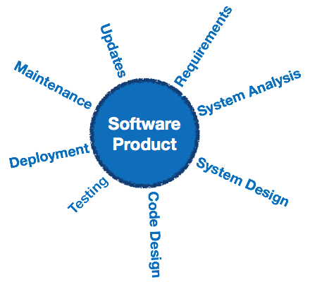
    The process of developing a software product using software engineering principles and methods is referred to as software evolution. This includes the initial development of software and its maintenance and updates, till desired software product is developed, which satisfies the expected requirements.

    Software Evolution

    Evolution starts from the requirement gathering process. After which developers create a prototype of the intended software and show it to the users to get their feedback at the early stage of software product development. The users suggest changes, on which several consecutive updates and maintenance keep on changing too. This process changes to the original software, till the desired software is accomplished.

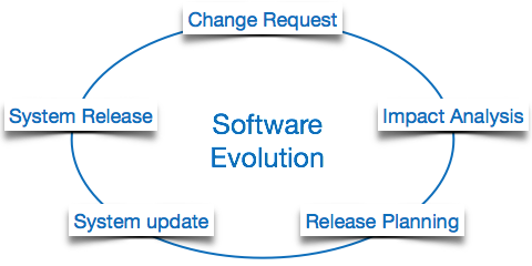
    Even after the user has desired software in hand, the advancing technology and the changing requirements force the software product to change accordingly. Re-creating software from scratch and to go one-on-one with requirement is not feasible. The only feasible and economical solution is to update the existing software so that it matches the latest requirements.

    Software Evolution Laws

    Lehman has given laws for software evolution. He divided the software into three different categories:

    • S-type (static-type) – This is a software, which works strictly according to defined specifications and solutions. The solution and the method to achieve it, both are immediately understood before coding. The s-type software is least subjected to changes hence this is the simplest of all. For example, calculator program for mathematical computation.
    • P-type (practical-type) – This is a software with a collection of procedures. This is defined by exactly what procedures can do. In this software, the specifications can be described but the solution is not obvious instantly. For example, gaming software.
    • E-type (embedded-type) – This software works closely as the requirement of real-world environment. This software has a high degree of evolution as there are various changes in laws, taxes etc. in the real world situations. For example, Online trading software.

    E-Type software evolution

    Lehman has given eight laws for E-Type software evolution –

    • Continuing change – An E-type software system must continue to adapt to the real world changes, else it becomes progressively less useful.
    • Increasing complexity – As an E-type software system evolves, its complexity tends to increase unless work is done to maintain or reduce it.
    • Conservation of familiarity – The familiarity with the software or the knowledge about how it was developed, why was it developed in that particular manner etc. must be retained at any cost, to implement the changes in the system.
    • Continuing growth- In order for an E-type system intended to resolve some business problem, its size of implementing the changes grows according to the lifestyle changes of the business.
    • Reducing quality – An E-type software system declines in quality unless rigorously maintained and adapted to a changing operational environment.
    • Feedback systems- The E-type software systems constitute multi-loop, multi-level feedback systems and must be treated as such to be successfully modified or improved.
    • Self-regulation – E-type system evolution processes are self-regulating with the distribution of product and process measures close to normal.
    • Organizational stability – The average effective global activity rate in an evolving E-type system is invariant over the lifetime of the product.

    Software Paradigms

    Software paradigms refer to the methods and steps, which are taken while designing the software. There are many methods proposed and are in work today, but we need to see where in the software engineering these paradigms stand. These can be combined into various categories, though each of them is contained in one another:

    Software Evolution

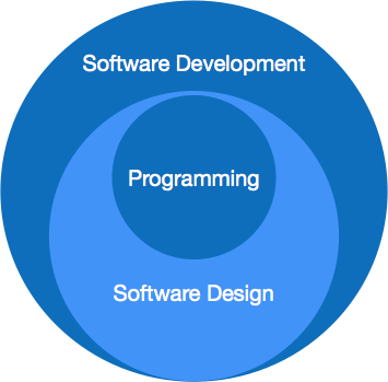
    Programming paradigm is a subset of Software design paradigm which is further a subset of Software development paradigm.

    Software Development Paradigm

    This Paradigm is known as software engineering paradigms where all the engineering concepts pertaining to the development of software are applied. It includes various researches and requirement gathering which helps the software product to build. It consists of

    • Requirement gathering
    • Software design
    • Programming

    Software Design Paradigm

    This paradigm is a part of Software Development and includes

    • Design
    • Maintenance
    • Programming

    Programming Paradigm

    This paradigm is related closely to programming aspect of software development. This includes

    • Coding
    • Testing
    • Integration

    Need of Software Engineering

    The need of software engineering arises because of higher rate of change in user requirements and environment on which the software is working.

    • Large software – It is easier to build a wall than to a house or building, likewise, as the size of software become large engineering has to step to give it a scientific process.
    • Scalability- If the software process were not based on scientific and engineering concepts, it would be easier to re-create new software than to scale an existing one.
    • Cost- As hardware industry has shown its skills and huge manufacturing has lower down he price of computer and electronic hardware. But the cost of software remains high if proper process is not adapted.
    • Dynamic Nature- The always growing and adapting nature of software hugely depends upon the environment in which user works. If the nature of software is always changing, new enhancements need to be done in the existing one. This is where software engineering plays a good role.
    • Quality Management- Better process of software development provides better and quality software product.

    Characteristics of good software

    A software product can be judged by what it offers and how well it can be used. This software must satisfy on the following grounds:

    • Operational
    • Transitional
    • Maintenance

    Well-engineered and crafted software is expected to have the following characteristics:

    Operational

    This tells us how well software works in operations. It can be measured on:

    • Budget
    • Usability
    • Efficiency
    • Correctness
    • Functionality
    • Dependability
    • Security
    • Safety

    Transitional

    This aspect is important when the software is moved from one platform to another:

    • Portability
    • Interoperability
    • Reusability
    • Adaptability

    Maintenance

    This aspect briefs about how well a software has the capabilities to maintain itself in the ever-changing environment:

    • Modularity
    • Maintainability
    • Flexibility
    • Scalability

    In short, Software engineering is a branch of computer science, which uses well-defined engineering concepts required to produce efficient, durable, scalable, in-budget and on-time software products.

  • Data Recovery

    DBMS is a highly complex system with hundreds of transactions being executed every second. The durability and robustness of a DBMS depends on its complex architecture and its underlying hardware and system software. If it fails or crashes amid transactions, it is expected that the system would follow some sort of algorithm or techniques to recover lost data.

    Failure Classification

    To see where the problem has occurred, we generalize a failure into various categories, as follows −

    Transaction failure

    A transaction has to abort when it fails to execute or when it reaches a point from where it cant go any further. This is called transaction failure where only a few transactions or processes are hurt.

    Reasons for a transaction failure could be −

    • Logical errors − Where a transaction cannot complete because it has some code error or any internal error condition.
    • System errors − Where the database system itself terminates an active transaction because the DBMS is not able to execute it, or it has to stop because of some system condition. For example, in case of deadlock or resource unavailability, the system aborts an active transaction.

    System Crash

    There are problems − external to the system − that may cause the system to stop abruptly and cause the system to crash. For example, interruptions in power supply may cause the failure of underlying hardware or software failure.

    Examples may include operating system errors.

    Disk Failure

    In early days of technology evolution, it was a common problem where hard-disk drives or storage drives used to fail frequently.

    Disk failures include formation of bad sectors, unreachability to the disk, disk head crash or any other failure, which destroys all or a part of disk storage.

    Storage Structure

    We have already described the storage system. In brief, the storage structure can be divided into two categories −

    • Volatile storage − As the name suggests, a volatile storage cannot survive system crashes. Volatile storage devices are placed very close to the CPU; normally they are embedded onto the chipset itself. For example, main memory and cache memory are examples of volatile storage. They are fast but can store only a small amount of information.
    • Non-volatile storage − These memories are made to survive system crashes. They are huge in data storage capacity, but slower in accessibility. Examples may include hard-disks, magnetic tapes, flash memory, and non-volatile (battery backed up) RAM.

    Recovery and Atomicity

    When a system crashes, it may have several transactions being executed and various files opened for them to modify the data items. Transactions are made of various operations, which are atomic in nature. But according to ACID properties of DBMS, atomicity of transactions as a whole must be maintained, that is, either all the operations are executed or none.

    When a DBMS recovers from a crash, it should maintain the following −

    • It should check the states of all the transactions, which were being executed.
    • A transaction may be in the middle of some operation; the DBMS must ensure the atomicity of the transaction in this case.
    • It should check whether the transaction can be completed now or it needs to be rolled back.
    • No transactions would be allowed to leave the DBMS in an inconsistent state.

    There are two types of techniques, which can help a DBMS in recovering as well as maintaining the atomicity of a transaction −

    • Maintaining the logs of each transaction, and writing them onto some stable storage before actually modifying the database.
    • Maintaining shadow paging, where the changes are done on a volatile memory, and later, the actual database is updated.

    Log-based Recovery

    Log is a sequence of records, which maintains the records of actions performed by a transaction. It is important that the logs are written prior to the actual modification and stored on a stable storage media, which is failsafe.

    Log-based recovery works as follows −

    • The log file is kept on a stable storage media.
    • When a transaction enters the system and starts execution, it writes a log about it.
    <Tn, Start>
    
    • When the transaction modifies an item X, it write logs as follows −
    <Tn, X, V1, V2>
    

    It reads Tn has changed the value of X, from V1 to V2.

    • When the transaction finishes, it logs −
    <Tn, commit>
    

    The database can be modified using two approaches −

    • Deferred database modification − All logs are written on to the stable storage and the database is updated when a transaction commits.
    • Immediate database modification − Each log follows an actual database modification. That is, the database is modified immediately after every operation.

    Recovery with Concurrent Transactions

    When more than one transaction are being executed in parallel, the logs are interleaved. At the time of recovery, it would become hard for the recovery system to backtrack all logs, and then start recovering. To ease this situation, most modern DBMS use the concept of ‘checkpoints’.

    Checkpoint

    Keeping and maintaining logs in real time and in real environment may fill out all the memory space available in the system. As time passes, the log file may grow too big to be handled at all. Checkpoint is a mechanism where all the previous logs are removed from the system and stored permanently in a storage disk. Checkpoint declares a point before which the DBMS was in consistent state, and all the transactions were committed.

    Recovery

    When a system with concurrent transactions crashes and recovers, it behaves in the following manner −

    Recovery
    • The recovery system reads the logs backwards from the end to the last checkpoint.
    • It maintains two lists, an undo-list and a redo-list.
    • If the recovery system sees a log with <Tn, Start> and <Tn, Commit> or just <Tn, Commit>, it puts the transaction in the redo-list.
    • If the recovery system sees a log with <Tn, Start> but no commit or abort log found, it puts the transaction in undo-list.

    All the transactions in the undo-list are then undone and their logs are removed. All the transactions in the redo-list and their previous logs are removed and then redone before saving their logs.

  • Data Backup

    Loss of Volatile Storage

    A volatile storage like RAM stores all the active logs, disk buffers, and related data. In addition, it stores all the transactions that are being currently executed. What happens if such a volatile storage crashes abruptly? It would obviously take away all the logs and active copies of the database. It makes recovery almost impossible, as everything that is required to recover the data is lost.

    Following techniques may be adopted in case of loss of volatile storage −

    • We can have checkpoints at multiple stages so as to save the contents of the database periodically.
    • A state of active database in the volatile memory can be periodically dumped onto a stable storage, which may also contain logs and active transactions and buffer blocks.
    • <dump> can be marked on a log file, whenever the database contents are dumped from a non-volatile memory to a stable one.

    Recovery

    • When the system recovers from a failure, it can restore the latest dump.
    • It can maintain a redo-list and an undo-list as checkpoints.
    • It can recover the system by consulting undo-redo lists to restore the state of all transactions up to the last checkpoint.

    Database Backup & Recovery from Catastrophic Failure

    A catastrophic failure is one where a stable, secondary storage device gets corrupt. With the storage device, all the valuable data that is stored inside is lost. We have two different strategies to recover data from such a catastrophic failure −

    • Remote backup &minu; Here a backup copy of the database is stored at a remote location from where it can be restored in case of a catastrophe.
    • Alternatively, database backups can be taken on magnetic tapes and stored at a safer place. This backup can later be transferred onto a freshly installed database to bring it to the point of backup.

    Grown-up databases are too bulky to be frequently backed up. In such cases, we have techniques where we can restore a database just by looking at its logs. So, all that we need to do here is to take a backup of all the logs at frequent intervals of time. The database can be backed up once a week, and the logs being very small can be backed up every day or as frequently as possible.

    Remote Backup

    Remote backup provides a sense of security in case the primary location where the database is located gets destroyed. Remote backup can be offline or real-time or online. In case it is offline, it is maintained manually.

    Remote Data Backup

    Online backup systems are more real-time and lifesavers for database administrators and investors. An online backup system is a mechanism where every bit of the real-time data is backed up simultaneously at two distant places. One of them is directly connected to the system and the other one is kept at a remote place as backup.

    As soon as the primary database storage fails, the backup system senses the failure and switches the user system to the remote storage. Sometimes this is so instant that the users cant even realize a failure.

  • Deadlock

    In a multi-process system, deadlock is an unwanted situation that arises in a shared resource environment, where a process indefinitely waits for a resource that is held by another process.

    For example, assume a set of transactions {T0, T1, T2, …,Tn}. T0 needs a resource X to complete its task. Resource X is held by T1, and T1 is waiting for a resource Y, which is held by T2. T2 is waiting for resource Z, which is held by T0. Thus, all the processes wait for each other to release resources. In this situation, none of the processes can finish their task. This situation is known as a deadlock.

    Deadlocks are not healthy for a system. In case a system is stuck in a deadlock, the transactions involved in the deadlock are either rolled back or restarted.

    Deadlock Prevention

    To prevent any deadlock situation in the system, the DBMS aggressively inspects all the operations, where transactions are about to execute. The DBMS inspects the operations and analyzes if they can create a deadlock situation. If it finds that a deadlock situation might occur, then that transaction is never allowed to be executed.

    There are deadlock prevention schemes that use timestamp ordering mechanism of transactions in order to predetermine a deadlock situation.

    Wait-Die Scheme

    In this scheme, if a transaction requests to lock a resource (data item), which is already held with a conflicting lock by another transaction, then one of the two possibilities may occur −

    • If TS(Ti) < TS(Tj) − that is Ti, which is requesting a conflicting lock, is older than Tj − then Ti is allowed to wait until the data-item is available.
    • If TS(Ti) > TS(tj) − that is Ti is younger than Tj − then Ti dies. Ti is restarted later with a random delay but with the same timestamp.

    This scheme allows the older transaction to wait but kills the younger one.

    Wound-Wait Scheme

    In this scheme, if a transaction requests to lock a resource (data item), which is already held with conflicting lock by some another transaction, one of the two possibilities may occur −

    • If TS(Ti) < TS(Tj), then Ti forces Tj to be rolled back − that is Ti wounds Tj. Tj is restarted later with a random delay but with the same timestamp.
    • If TS(Ti) > TS(Tj), then Ti is forced to wait until the resource is available.

    This scheme, allows the younger transaction to wait; but when an older transaction requests an item held by a younger one, the older transaction forces the younger one to abort and release the item.

    In both the cases, the transaction that enters the system at a later stage is aborted.

    Deadlock Avoidance

    Aborting a transaction is not always a practical approach. Instead, deadlock avoidance mechanisms can be used to detect any deadlock situation in advance. Methods like “wait-for graph” are available but they are suitable for only those systems where transactions are lightweight having fewer instances of resource. In a bulky system, deadlock prevention techniques may work well.

    Wait-for Graph

    This is a simple method available to track if any deadlock situation may arise. For each transaction entering into the system, a node is created. When a transaction Ti requests for a lock on an item, say X, which is held by some other transaction Tj, a directed edge is created from Ti to Tj. If Tj releases item X, the edge between them is dropped and Ti locks the data item.

    The system maintains this wait-for graph for every transaction waiting for some data items held by others. The system keeps checking if there’s any cycle in the graph.

    Wait-for Graph

    Here, we can use any of the two following approaches −

    • First, do not allow any request for an item, which is already locked by another transaction. This is not always feasible and may cause starvation, where a transaction indefinitely waits for a data item and can never acquire it.
    • The second option is to roll back one of the transactions. It is not always feasible to roll back the younger transaction, as it may be important than the older one. With the help of some relative algorithm, a transaction is chosen, which is to be aborted. This transaction is known as the victim and the process is known as victim selection.
  • Concurrency Control

    In a multiprogramming environment where multiple transactions can be executed simultaneously, it is highly important to control the concurrency of transactions. We have concurrency control protocols to ensure atomicity, isolation, and serializability of concurrent transactions. Concurrency control protocols can be broadly divided into two categories −

    • Lock based protocols
    • Time stamp based protocols

    Lock-based Protocols

    Database systems equipped with lock-based protocols use a mechanism by which any transaction cannot read or write data until it acquires an appropriate lock on it. Locks are of two kinds −

    • Binary Locks − A lock on a data item can be in two states; it is either locked or unlocked.
    • Shared/exclusive − This type of locking mechanism differentiates the locks based on their uses. If a lock is acquired on a data item to perform a write operation, it is an exclusive lock. Allowing more than one transaction to write on the same data item would lead the database into an inconsistent state. Read locks are shared because no data value is being changed.

    There are four types of lock protocols available −

    Simplistic Lock Protocol

    Simplistic lock-based protocols allow transactions to obtain a lock on every object before a ‘write’ operation is performed. Transactions may unlock the data item after completing the write operation.

    Pre-claiming Lock Protocol

    Pre-claiming protocols evaluate their operations and create a list of data items on which they need locks. Before initiating an execution, the transaction requests the system for all the locks it needs beforehand. If all the locks are granted, the transaction executes and releases all the locks when all its operations are over. If all the locks are not granted, the transaction rolls back and waits until all the locks are granted.

    Pre-claiming

    Two-Phase Locking 2PL

    This locking protocol divides the execution phase of a transaction into three parts. In the first part, when the transaction starts executing, it seeks permission for the locks it requires. The second part is where the transaction acquires all the locks. As soon as the transaction releases its first lock, the third phase starts. In this phase, the transaction cannot demand any new locks; it only releases the acquired locks.

    Two Phase Locking

    Two-phase locking has two phases, one is growing, where all the locks are being acquired by the transaction; and the second phase is shrinking, where the locks held by the transaction are being released.

    To claim an exclusive (write) lock, a transaction must first acquire a shared (read) lock and then upgrade it to an exclusive lock.

    Strict Two-Phase Locking

    The first phase of Strict-2PL is same as 2PL. After acquiring all the locks in the first phase, the transaction continues to execute normally. But in contrast to 2PL, Strict-2PL does not release a lock after using it. Strict-2PL holds all the locks until the commit point and releases all the locks at a time.

    Strict Two Phase Locking

    Strict-2PL does not have cascading abort as 2PL does.

    Timestamp-based Protocols

    The most commonly used concurrency protocol is the timestamp based protocol. This protocol uses either system time or logical counter as a timestamp.

    Lock-based protocols manage the order between the conflicting pairs among transactions at the time of execution, whereas timestamp-based protocols start working as soon as a transaction is created.

    Every transaction has a timestamp associated with it, and the ordering is determined by the age of the transaction. A transaction created at 0002 clock time would be older than all other transactions that come after it. For example, any transaction ‘y’ entering the system at 0004 is two seconds younger and the priority would be given to the older one.

    In addition, every data item is given the latest read and write-timestamp. This lets the system know when the last read and write operation was performed on the data item.

    Timestamp Ordering Protocol

    The timestamp-ordering protocol ensures serializability among transactions in their conflicting read and write operations. This is the responsibility of the protocol system that the conflicting pair of tasks should be executed according to the timestamp values of the transactions.

    • The timestamp of transaction Ti is denoted as TS(Ti).
    • Read time-stamp of data-item X is denoted by R-timestamp(X).
    • Write time-stamp of data-item X is denoted by W-timestamp(X).

    Timestamp ordering protocol works as follows −

    • If a transaction Ti issues a read(X) operation −
      • If TS(Ti) < W-timestamp(X)
        • Operation rejected.
      • If TS(Ti) >= W-timestamp(X)
        • Operation executed.
      • All data-item timestamps updated.
    • If a transaction Ti issues a write(X) operation −
      • If TS(Ti) < R-timestamp(X)
        • Operation rejected.
      • If TS(Ti) < W-timestamp(X)
        • Operation rejected and Ti rolled back.
      • Otherwise, operation executed.

    Thomas’ Write Rule

    This rule states if TS(Ti) < W-timestamp(X), then the operation is rejected and Ti is rolled back.

    Time-stamp ordering rules can be modified to make the schedule view serializable.

    Instead of making Ti rolled back, the ‘write’ operation itself is ignored.

  • Transaction

    A transaction can be defined as a group of tasks. A single task is the minimum processing unit which cannot be divided further.

    Lets take an example of a simple transaction. Suppose a bank employee transfers Rs 500 from A’s account to B’s account. This very simple and small transaction involves several low-level tasks.

    As Account

    Open_Account(A)
    Old_Balance = A.balance
    New_Balance = Old_Balance - 500
    A.balance = New_Balance
    Close_Account(A)
    

    Bs Account

    Open_Account(B)
    Old_Balance = B.balance
    New_Balance = Old_Balance + 500
    B.balance = New_Balance
    Close_Account(B)
    

    ACID Properties

    A transaction is a very small unit of a program and it may contain several lowlevel tasks. A transaction in a database system must maintain Atomicity, Consistency, Isolation, and Durability − commonly known as ACID properties − in order to ensure accuracy, completeness, and data integrity.

    • Atomicity − This property states that a transaction must be treated as an atomic unit, that is, either all of its operations are executed or none. There must be no state in a database where a transaction is left partially completed. States should be defined either before the execution of the transaction or after the execution/abortion/failure of the transaction.
    • Consistency − The database must remain in a consistent state after any transaction. No transaction should have any adverse effect on the data residing in the database. If the database was in a consistent state before the execution of a transaction, it must remain consistent after the execution of the transaction as well.
    • Durability − The database should be durable enough to hold all its latest updates even if the system fails or restarts. If a transaction updates a chunk of data in a database and commits, then the database will hold the modified data. If a transaction commits but the system fails before the data could be written on to the disk, then that data will be updated once the system springs back into action.
    • Isolation − In a database system where more than one transaction are being executed simultaneously and in parallel, the property of isolation states that all the transactions will be carried out and executed as if it is the only transaction in the system. No transaction will affect the existence of any other transaction.

    Serializability

    When multiple transactions are being executed by the operating system in a multiprogramming environment, there are possibilities that instructions of one transactions are interleaved with some other transaction.

    • Schedule − A chronological execution sequence of a transaction is called a schedule. A schedule can have many transactions in it, each comprising of a number of instructions/tasks.
    • Serial Schedule − It is a schedule in which transactions are aligned in such a way that one transaction is executed first. When the first transaction completes its cycle, then the next transaction is executed. Transactions are ordered one after the other. This type of schedule is called a serial schedule, as transactions are executed in a serial manner.

    In a multi-transaction environment, serial schedules are considered as a benchmark. The execution sequence of an instruction in a transaction cannot be changed, but two transactions can have their instructions executed in a random fashion. This execution does no harm if two transactions are mutually independent and working on different segments of data; but in case these two transactions are working on the same data, then the results may vary. This ever-varying result may bring the database to an inconsistent state.

    To resolve this problem, we allow parallel execution of a transaction schedule, if its transactions are either serializable or have some equivalence relation among them.

    Equivalence Schedules

    An equivalence schedule can be of the following types −

    Result Equivalence

    If two schedules produce the same result after execution, they are said to be result equivalent. They may yield the same result for some value and different results for another set of values. That’s why this equivalence is not generally considered significant.

    View Equivalence

    Two schedules would be view equivalence if the transactions in both the schedules perform similar actions in a similar manner.

    For example −

    • If T reads the initial data in S1, then it also reads the initial data in S2.
    • If T reads the value written by J in S1, then it also reads the value written by J in S2.
    • If T performs the final write on the data value in S1, then it also performs the final write on the data value in S2.

    Conflict Equivalence

    Two schedules would be conflicting if they have the following properties −

    • Both belong to separate transactions.
    • Both accesses the same data item.
    • At least one of them is “write” operation.

    Two schedules having multiple transactions with conflicting operations are said to be conflict equivalent if and only if −

    • Both the schedules contain the same set of Transactions.
    • The order of conflicting pairs of operation is maintained in both the schedules.

    Note − View equivalent schedules are view serializable and conflict equivalent schedules are conflict serializable. All conflict serializable schedules are view serializable too.

    States of Transactions

    A transaction in a database can be in one of the following states −

    Transaction States
    • Active − In this state, the transaction is being executed. This is the initial state of every transaction.
    • Partially Committed − When a transaction executes its final operation, it is said to be in a partially committed state.
    • Failed − A transaction is said to be in a failed state if any of the checks made by the database recovery system fails. A failed transaction can no longer proceed further.
    • Aborted − If any of the checks fails and the transaction has reached a failed state, then the recovery manager rolls back all its write operations on the database to bring the database back to its original state where it was prior to the execution of the transaction. Transactions in this state are called aborted. The database recovery module can select one of the two operations after a transaction aborts −
      • Re-start the transaction
      • Kill the transaction
    • Committed − If a transaction executes all its operations successfully, it is said to be committed. All its effects are now permanently established on the database system.
  • Hashing

    For a huge database structure, it can be almost next to impossible to search all the index values through all its level and then reach the destination data block to retrieve the desired data. Hashing is an effective technique to calculate the direct location of a data record on the disk without using index structure.

    Hashing uses hash functions with search keys as parameters to generate the address of a data record.

    Hash Organization

    • Bucket − A hash file stores data in bucket format. Bucket is considered a unit of storage. A bucket typically stores one complete disk block, which in turn can store one or more records.
    • Hash Function − A hash function, h, is a mapping function that maps all the set of search-keys K to the address where actual records are placed. It is a function from search keys to bucket addresses.

    Static Hashing

    In static hashing, when a search-key value is provided, the hash function always computes the same address. For example, if mod-4 hash function is used, then it shall generate only 5 values. The output address shall always be same for that function. The number of buckets provided remains unchanged at all times.

    Static Hashing

    Operation

    • Insertion − When a record is required to be entered using static hash, the hash function h computes the bucket address for search key K, where the record will be stored.Bucket address = h(K)
    • Search − When a record needs to be retrieved, the same hash function can be used to retrieve the address of the bucket where the data is stored.
    • Delete − This is simply a search followed by a deletion operation.

    Bucket Overflow

    The condition of bucket-overflow is known as collision. This is a fatal state for any static hash function. In this case, overflow chaining can be used.

    • Overflow Chaining − When buckets are full, a new bucket is allocated for the same hash result and is linked after the previous one. This mechanism is called Closed Hashing.
    Overflow chaining
    • Linear Probing − When a hash function generates an address at which data is already stored, the next free bucket is allocated to it. This mechanism is called Open Hashing.
    Linear Probing

    Dynamic Hashing

    The problem with static hashing is that it does not expand or shrink dynamically as the size of the database grows or shrinks. Dynamic hashing provides a mechanism in which data buckets are added and removed dynamically and on-demand. Dynamic hashing is also known as extended hashing.

    Hash function, in dynamic hashing, is made to produce a large number of values and only a few are used initially.

    Dynamic Hashing

    Organization

    The prefix of an entire hash value is taken as a hash index. Only a portion of the hash value is used for computing bucket addresses. Every hash index has a depth value to signify how many bits are used for computing a hash function. These bits can address 2n buckets. When all these bits are consumed − that is, when all the buckets are full − then the depth value is increased linearly and twice the buckets are allocated.

    Operation

    • Querying − Look at the depth value of the hash index and use those bits to compute the bucket address.
    • Update − Perform a query as above and update the data.
    • Deletion − Perform a query to locate the desired data and delete the same.
    • Insertion − Compute the address of the bucket
      • If the bucket is already full.
        • Add more buckets.
        • Add additional bits to the hash value.
        • Re-compute the hash function.
      • Else
        • Add data to the bucket,
      • If all the buckets are full, perform the remedies of static hashing.

    Hashing is not favorable when the data is organized in some ordering and the queries require a range of data. When data is discrete and random, hash performs the best.

    Hashing algorithms have high complexity than indexing. All hash operations are done in constant time.

  • Dynamic Multilevel Indexing with B-Tree and B+ Tree

    Large databases require efficient methods for indexing. It is crucial that we maintain proper indexes to search records in large databases. A common challenge is to make sure the index structure remains balanced when new records are inserted or existing ones are deleted. For this purpose, there are different methods like single level indexing, multi-level indexing, and dynamic multilevel indexing.

    Multilevel indexing can be done using B-Trees and B+ Trees. These advanced data structures adjust themselves automatically, keeping the operations smooth and fast. Read this chapter to learn the fundamentals of dynamic multilevel indexing and understand how B-Trees and B+ Trees work.

    What is Dynamic Multilevel Indexing?

    Dynamic multilevel indexing helps in maintaining an efficient search structure. This is true even when the records in a database keep changing frequently. Unlike static indexing where we can update by rebuilding the index, dynamic indexing updates itself on the fly.

    The two most common structures used are B- Trees and B+ Trees. Both work as balanced tree structures. These trees keep the search times short by minimizing the number of levels. They handle insertions, deletions, and searches efficiently, even in large datasets.

    The Role of B- Trees in Dynamic Indexing

    B- Tree is a balanced search tree where records are stored within its nodes. Each node contains multiple key values and pointers to other nodes or records. The key idea is to keep the tree balanced by splitting and merging the nodes as records are inserted or deleted.

    How Does a B- Tree Work?

    Let’s understand how a B-Tree works −

    • Nodes and Keys − Each node can have several keys and pointers that form a multi-way search tree.
    • Balanced Structure − The tree is always balanced, which means every leaf node is at the same level.
    • Search Process − The search begins at the root and follows pointers based on key comparisons until the desired record is found.

    The following image depicts how a B-Tree looks like −

    Role of B- Trees in Dynamic Indexing

    Key Properties of B-Trees

    Given below are some of the important properties of B-Trees −

    • Every internal node can have up to “p – 1” keys and “p” pointers. Here, “p” is the order of the B-Tree.
    • Keys in each node are arranged in ascending order.
    • Each node must be at least half full, except for the root.
    • Leaf nodes are linked for easier traversal if needed.

    Example of a B-Tree

    Let’s see an example of a B-Tree for a database with order and fan-out −

    • Order (p) − 23 (maximum keys a node can hold)
    • Fan-out (fo) − 16 (average number of pointers in a node)

    We start with the root node that holds 15 key entries and 16 pointers. As new records are inserted, the tree grows as follows −

    • Level 0 (Root) − 1 node with 15 keys and 16 pointers
    • Level 1 − 16 nodes with 240 keys and 256 pointers
    • Level 2 − 256 nodes with 3840 keys and 4096 pointers
    • Level 3 (Leaf Level) − 4096 nodes holding 61,440 keys

    The tree can efficiently organize over 65,535 records and we can see that there are just three levels. It is this efficiency that reduces the search times to a great extent.

    B+ Trees: More Efficient than B-Tree

    A B+ Tree is a modified version of a B-Tree. B+ Trees are specifically designed for indexing. In a B+ Tree, all the data records are stored only at the leaf nodes and the internal nodes hold only keys and pointers. This design allows the internal nodes to hold more keys, making the structure shallower and more efficient.

    How Do B+ Trees Work

    In a B+ Tree,

    • Leaf Nodes − Contain records or pointers to records.
    • Internal Nodes − Contain only keys and pointers to lower-level nodes.
    • Linked Leaf Nodes − Leaf nodes are linked, which makes the sequential access easier.

    Key Properties of B+ Trees

    Listed below are some of the important properties of B+ Trees −

    • Every internal node can have up to p pointers and p-1 keys.
    • Leaf nodes hold actual data or pointers to data.
    • Leaf nodes are linked for easy traversal.
    • The tree stays balanced due to automatic splitting and merging during updates.

    Example of a B+ Tree

    Let us see the same example that we used for explaining B-Trees but this time, with B+ Tree logic −

    Assumptions −

    • Key size − 9 bytes
    • Pointer size − 7 bytes (for records), 6 bytes (for blocks)
    • Block size − 512 bytes

    Internal Nodes − Maximum of 34 keys and 35 pointers (calculated based on available space).

    Leaf Nodes − Maximum of 31 data entries (keys and data pointers).

    • Root Node − 1 node with 22 keys and 23 pointers.
    • Level 1 − 23 nodes holding 506 keys and 529 pointers.
    • Level 2 − 529 nodes holding 11,638 keys and 12,167 pointers.
    • Leaf Level − 12,167 nodes holding 255,507 data pointers.

    This structure is useful and it can handle over 255,507 records efficiently with just three levels. This is why B+ Trees are commonly used in database indexing systems.

    Advantages of Dynamic Multilevel Indexing

    Dynamic multilevel indexing offers several advantages as given below −

    • Automatic Balancing − Trees adjust themselves during insertions and deletions.
    • Efficient Searches − Shallow trees mean fewer levels to search through.
    • Faster Updates − Data changes are quick due to rebalancing logic.
    • Scalability − B-Trees and B+ Trees handle massive datasets without performance drops.

    Real-world Applications of B-Trees and B+ Trees

    B-Trees and B+ Trees are widely used in −

    • DBMS − For indexing large tables.
    • File Systems − To manage files in storage systems.
    • Search Engines − To keep search indexes optimized.
    • Operating Systems − For directory management.

    Difference between B-Trees and B+ Trees

    The following table highlights the major differences between B-Trees and B+ Trees −

    FeatureB- TreeB+ Tree
    Data StorageIn all nodesOnly in leaf nodes
    Data RetrievalSlower for range queriesFaster due to linked leaf nodes
    Tree DepthDeeperShallower
    Use CasesGeneral indexingIndexing with range queries
  • Multi-level Indexing

    Data retrieval is the process in database management systems where we need speed and efficiency. We implement the concept of indexing in order to reduce the search time and facilitate faster data retrieval. As databases grow in size, efficient indexing techniques become our primary option to reduce search times. Multi-level indexing is one such indexing technique that is designed to manage large datasets with minimal disk access. Read this chapter to get a good understanding of what multi-level indexing means, what is its structure, and how it works.

    What is Multi-level Indexing in DBMS?

    In database systems, indexing improves the data retrieval speed by organizing the records in a way that allows faster searches. A single-level index makes a list of key values pointing to corresponding records. This process can be used with a binary search. However, when we are working with massive datasets, a single-level index becomes inefficient due to its size. This is where multi-level indexing is needed for efficiency.

    Why Do We Use Multi-level Indexing?

    The main reason for using multi-level indexing is to reduce the number of blocks accessed during a search. We know we can apply the binary search where the search space is divided in half at each step. Binary search requires approximately log2 (bi) block accesses for an index with bi blocks. With multi-level indexing, we can improve the search speed by dividing the search space into larger segments. It will reduce the search time exponentially.

    For example, instead of cutting the search space in half, we can use multi-level indexing to split it further. This reduces the search space by a factor equal to the fan-out (f0) value, which denotes the number of entries that can fit into a single block. When the fan-out value is much larger than 2, the search process becomes significantly faster.

    Structure of Multi-level Indexing

    To understand the concept of multi-level indexing, we must know its structures. It is organized into different levels, each representing a progressively smaller index until a manageable size is reached.

    The structure consists of −

    • First Level (Base Level) − This level stores the main index entries. This is also called the base index. It contains unique key values and pointers to corresponding records.
    • Second Level − This level acts as a primary index for the first level. It stores pointers to the blocks of the first level.
    • Higher Levels − If the second level becomes too large to fit in a single block, then additional levels are created. It reduces the index size further.
    Structure of Multi-level Indexing

    How Does Multi-level Indexing Work?

    Each level of the multi-level index reduces the number of entries in the previous level. This is done by the fan-out value (f0). The process continues until the final level fits into a single block, referred to as the top level.

    The number of levels (t) required is calculated as −

    t=[logf0(r1)]

    Where, r1 is the number of entries in the first level and f0 is the fan-out value.

    From this, it is evident that searching involves retrieving a block from each level and finally accessing the data block. It results in a total of t + 1 block accesses.

    Example of Multi-level Indexing

    Let us take a detailed example to understand multi-level indexing in action.

    The given data is as follows −

    • Blocking factor (bfri) − 68 entries per block (also called the fan-out, fo).
    • First-level blocks (b1) − 442 blocks.

    Step 1: Calculate the Second Level

    We calculate the number of blocks needed at the second level −

    b2=[b1f0]=[44268]=7

    The second level has seven blocks.

    Step 2: Calculate the Third Level

    Similarly, we can calculate the number of blocks needed at the third level −

    b3=[b2f0]=[768]=1

    Since the third level fits into one block, it becomes the top level of the index. This is making the total number of levels t = 3.

    Step 3: Record Search Example

    After making the index, we must search from it. To search for a record using this multi-level index, we need to access −

    • One block from each level − Three levels in total.
    • One data block from the file − The block containing the record.

    Total Block Accesses is: T + 1 = 3 + 1 = 4. This is a significant improvement over a single-level index. There are 10 block accesses would have been needed using a binary search.

    Types of Multi-level Indexing

    Depending on the type of records and access patterns, multi-level indexing can be applied in various forms −

    • Primary Index − Built on a sorted key field, which makes it sparse (only one index entry per block).
    • Clustering Index − Built on non-key fields where multiple records share the same value.
    • Secondary Index − Built on unsorted fields, requiring more maintenance but offering flexibility.

    Indexed Sequential Access Method (ISAM)

    Indexed Sequential Access Method (ISAM) is a practical implementation of multi-level indexing. ISAM is commonly used in older IBM systems. It uses a two-level index −

    • Cylinder Index − Points to track-level blocks.
    • Track Index − Points to specific tracks in the cylinder.

    Data insertion is managed using overflow files. This is periodically merged with the main file during reorganization.

    Advantages of Multi-level Indexing

    Multi-level indexing offers the following benefits −

    • Faster Searches − Reduces the number of disk accesses.
    • Scalability − Handles large datasets efficiently.
    • Supports Different Index Types − Works with primary, clustering, and secondary indexes.
    • Balanced Access − Ensures near-uniform access times.

    One of the major challenges in managing multi-level indexes is during insertions or deletions. It can be complex, as all index levels must be updated. This process becomes problematic when frequent updates occur.

    The solution could be dynamic indexing. To address this problem, modern databases use dynamic multi-level indexes such as B − trees and B+ − trees. These structures balance the index by reorganizing the nodes automatically during insertions and deletions.

  • Indexing

    We know that data is stored in the form of records. Every record has a key field, which helps it to be recognized uniquely.

    Indexing is a data structure technique to efficiently retrieve records from the database files based on some attributes on which the indexing has been done. Indexing in database systems is similar to what we see in books.

    Indexing is defined based on its indexing attributes. Indexing can be of the following types −

    • Primary Index − Primary index is defined on an ordered data file. The data file is ordered on a key field. The key field is generally the primary key of the relation.
    • Secondary Index − Secondary index may be generated from a field which is a candidate key and has a unique value in every record, or a non-key with duplicate values.
    • Clustering Index − Clustering index is defined on an ordered data file. The data file is ordered on a non-key field.

    Ordered Indexing is of two types −

    • Dense Index
    • Sparse Index

    Dense Index

    In dense index, there is an index record for every search key value in the database. This makes searching faster but requires more space to store index records itself. Index records contain search key value and a pointer to the actual record on the disk.

    Dense Index

    Sparse Index

    In sparse index, index records are not created for every search key. An index record here contains a search key and an actual pointer to the data on the disk. To search a record, we first proceed by index record and reach at the actual location of the data. If the data we are looking for is not where we directly reach by following the index, then the system starts sequential search until the desired data is found.

    Sparse Index

    Multilevel Index

    Index records comprise search-key values and data pointers. Multilevel index is stored on the disk along with the actual database files. As the size of the database grows, so does the size of the indices. There is an immense need to keep the index records in the main memory so as to speed up the search operations. If single-level index is used, then a large size index cannot be kept in memory which leads to multiple disk accesses.

    Multi-level Index

    Multi-level Index helps in breaking down the index into several smaller indices in order to make the outermost level so small that it can be saved in a single disk block, which can easily be accommodated anywhere in the main memory.

    B+ Tree

    A B+ tree is a balanced binary search tree that follows a multi-level index format. The leaf nodes of a B+ tree denote actual data pointers. B+ tree ensures that all leaf nodes remain at the same height, thus balanced. Additionally, the leaf nodes are linked using a link list; therefore, a B+ tree can support random access as well as sequential access.

    Structure of B+ Tree

    Every leaf node is at equal distance from the root node. A B+ tree is of the order n where n is fixed for every B+ tree.

    B+ tree

    Internal nodes −

    • Internal (non-leaf) nodes contain at least ⌈n/2⌉ pointers, except the root node.
    • At most, an internal node can contain n pointers.

    Leaf nodes −

    • Leaf nodes contain at least ⌈n/2⌉ record pointers and ⌈n/2⌉ key values.
    • At most, a leaf node can contain n record pointers and n key values.
    • Every leaf node contains one block pointer P to point to next leaf node and forms a linked list.

    B+ Tree Insertion

    • B+ trees are filled from bottom and each entry is done at the leaf node.
    • If a leaf node overflows −
      • Split node into two parts.
      • Partition at i = ⌊(m+1)/2⌋.
      • First i entries are stored in one node.
      • Rest of the entries (i+1 onwards) are moved to a new node.
      • ith key is duplicated at the parent of the leaf.
    • If a non-leaf node overflows −
      • Split node into two parts.
      • Partition the node at i = ⌈(m+1)/2.
      • Entries up to i are kept in one node.
      • Rest of the entries are moved to a new node.

    B+ Tree Deletion

    • B+ tree entries are deleted at the leaf nodes.
    • The target entry is searched and deleted.
      • If it is an internal node, delete and replace with the entry from the left position.
    • After deletion, underflow is tested,
      • If underflow occurs, distribute the entries from the nodes left to it.
    • If distribution is not possible from left, then
      • Distribute from the nodes right to it.
    • If distribution is not possible from left or from right, then
      • Merge the node with left and right to it.