Author: saqibkhan

Linked List Basics

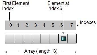
Linked List is a sequence of links which contains items. Each link contains a connection to another link. Linked list the second most used data structure after array. Following are important terms to understand the concepts of Linked List.

• Link − Each Link of a linked list can store a data called an element.
• Next − Each Link of a linked list contain a link to next link called Next.
• LinkedList − A LinkedList contains the connection link to the first Link called First.

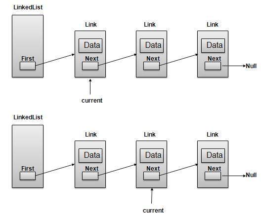
Linked List Representation

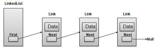
As per above shown illustration, following are the important points to be considered.

• LinkedList contains an link element called first.
• Each Link carries a data field(s) and a Link Field called next.
• Each Link is linked with its next link using its next link.
• Last Link carries a Link as null to mark the end of the list.

Learn Java in-depth with real-world projects through our Java certification course. Enroll and become a certified expert to boost your career.

Types of Linked List

Following are the various flavours of linked list.

• Simple Linked List − Item Navigation is forward only.
• Doubly Linked List − Items can be navigated forward and backward way.
• Circular Linked List − Last item contains link of the first element as next and and first element has link to last element as prev.

Basic Operations

Following are the basic operations supported by a list.

• Insertion − add an element at the beginning of the list.
• Deletion − delete an element at the beginning of the list.
• Display − displaying complete list.
• Search − search an element using given key.
• Delete − delete an element using given key.

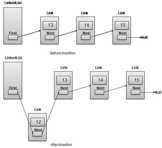
Insertion Operation

Insertion is a three step process:

1. Create a new Link with provided data.
2. Point New Link to old First Link.
3. Point First Link to this New Link.

//insert link at the first location
public void insertFirst(int key, int data){
   //create a link
   Link link = new Link(key,data);
   //point it to old first node
   link.next = first;
   //point first to new first node
   first = link;
}

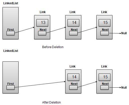
Deletion Operation

Deletion is a two step process:

1. Get the Link pointed by First Link as Temp Link.
2. Point First Link to Temp Link’s Next Link.

//delete first item
public Link deleteFirst(){
   //save reference to first link
   Link tempLink = first;
   //mark next to first link as first 
   first = first.next;
   //return the deleted link
   return tempLink;
}

Navigation Operation

Navigation is a recursive step process and is basis of many operations like search, delete etc.:

1. Get the Link pointed by First Link as Current Link.
2. Check if Current Link is not null and display it.
3. Point Current Link to Next Link of Current Link and move to above step.

Note

//display the list
public void display(){
   //start from the beginning
   Link current = first;
   //navigate till the end of the list
   System.out.print("[ ");
   while(current != null){
  //print data
  current.display();
  //move to next item
  current = current.next;
  System.out.print(" ");
   }
   System.out.print(" ]");
}

Advanced Operations

Following are the advanced operations specified for a list.

• Sort − sorting a list based on a particular order.
• Reverse − reversing a linked list.
• Concatenate − concatenate two lists.

Sort Operation

We’ve used bubble sort to sort a list.

public void sort(){

   int i, j, k, tempKey, tempData ;
   Link current,next;
   int size = length();
   k = size ;
   for ( i = 0 ; i < size - 1 ; i++, k-- ) {
  current = first ;
  next = first.next ;
  for ( j = 1 ; j &lt; k ; j++ ) {            
     if ( current.data &gt; next.data ) {
        tempData = current.data ;
        current.data = next.data;
        next.data = tempData ;
        tempKey = current.key;
        current.key = next.key;
        next.key = tempKey;
     }
     current = current.next;
     next = next.next;                        
  }
   }
}

Reverse Operation

Following code demonstrate reversing a single linked list.

public LinkedList reverse() { 
   LinkedList reversedlist = new LinkedList();
   Link nextLink = null;     
   reversedlist.insertFirst(first.key, first.data);

   Link currentLink = first;       
   // Until no more data in list, 
   // insert current link before first and move ahead.
   while(currentLink.next != null){
  nextLink = currentLink.next;           
  // Insert at start of new list.
  reversedlist.insertFirst(nextLink.key, nextLink.data); 
  //advance to next node
  currentLink = currentLink.next;            
   }      
   return reversedlist;
}

Concatenate Operation

Following code demonstrate reversing a single linked list.

public void concatenate(LinkedList list){
   if(first == null){
  first = list.first;
   }
   if(list.first == null){
  return;
   }
   Link temp = first;
   while(temp.next !=null) {
  temp = temp.next;
   }
   temp.next = list.first;       
}

Demo

Link.java

package com.tutorialspoint.list;

public class Link {
   public int key;
   public int data;
   public Link next;

   public Link(int key, int data){
  this.key = key;
  this.data = data;
   }

   public void display(){
  System.out.print("{"+key+","+data+"}");
   }
}

LinkedList.java

package com.tutorialspoint.list;

public class LinkedList {
   //this link always point to first Link 
   //in the Linked List 
   private Link first;

   // create an empty linked list 
   public LinkedList(){
  first = null;
   }

   //insert link at the first location
   public void insertFirst(int key, int data){
  //create a link
  Link link = new Link(key,data);
  //point it to old first node
  link.next = first;
  //point first to new first node
  first = link;
   }

   //delete first item
   public Link deleteFirst(){
  //save reference to first link
  Link tempLink = first;
  //mark next to first link as first 
  first = first.next;
  //return the deleted link
  return tempLink;
   }

   //display the list
   public void display(){
  //start from the beginning
  Link current = first;
  //navigate till the end of the list
  System.out.print("[ ");
  while(current != null){
     //print data
     current.display();
     //move to next item
     current = current.next;
     System.out.print(" ");
  }
  System.out.print(" ]");
   }

   //find a link with given key
   public Link find(int key){
  //start from the first link
  Link current = first;
  //if list is empty
  if(first == null){
     return null;
  }
  //navigate through list
  while(current.key != key){
     //if it is last node
     if(current.next == null){
        return null;
     }else{
        //go to next link
        current = current.next;
     }
  }      
  //if data found, return the current Link
  return current;
   }

   //delete a link with given key
   public Link delete(int key){
  //start from the first link
  Link current = first;
  Link previous = null;
  //if list is empty
  if(first == null){
     return null;
  }
  //navigate through list
  while(current.key != key){
     //if it is last node
     if(current.next == null){
        return null;
     }else{
        //store reference to current link
        previous = current;
        //move to next link
        current = current.next;             
     }
  }
  //found a match, update the link
  if(current == first) {
     //change first to point to next link
     first = first.next;
  }else {
     //bypass the current link
     previous.next = current.next;
  }    
  return current;
   }


   //is list empty
   public boolean isEmpty(){
  return first == null;
   }
   
   public int length(){
  int length = 0;
  for(Link current = first; current!=null;
     current = current.next){
     length++;
  }
  return length;
   }
   
   public void sort(){
  int i, j, k, tempKey, tempData ;
  Link current,next;
  int size = length();
  k = size ;
  for ( i = 0 ; i < size - 1 ; i++, k-- ) {
     current = first ;
     next = first.next ;
     for ( j = 1 ; j < k ; j++ ) {            
        if ( current.data > next.data ) {
           tempData = current.data ;
           current.data = next.data;
           next.data = tempData ;
	 
           tempKey = current.key;
           current.key = next.key;
           next.key = tempKey;
        }
        current = current.next;
       next = next.next;                        
     }
  }
   }

   public LinkedList reverse() { 
  LinkedList reversedlist = new LinkedList();
  Link nextLink = null;     
  reversedlist.insertFirst(first.key, first.data);
  Link currentLink = first;       
  // Until no more data in list, 
  // insert current link before first and move ahead.
  while(currentLink.next != null){
     nextLink = currentLink.next;           
     // Insert at start of new list.
     reversedlist.insertFirst(nextLink.key, nextLink.data); 
     //advance to next node
     currentLink = currentLink.next;            
  }      
  return reversedlist;
   }

   public void concatenate(LinkedList list){
  if(first == null){
     first = list.first;
  }
  if(list.first == null){
     return;
  }
  Link temp = first;
  while(temp.next !=null) {
     temp = temp.next;
  }
  temp.next = list.first;       
   }
}

LinkedListDemo.java

package com.tutorialspoint.list;

public class LinkedListDemo {
   public static void main(String args[]){
  LinkedList list = new LinkedList();
    
  list.insertFirst(1, 10);
  list.insertFirst(2, 20);
  list.insertFirst(3, 30);
  list.insertFirst(4, 1);
  list.insertFirst(5, 40);
  list.insertFirst(6, 56);
  System.out.print("\nOriginal List: ");  
  list.display();
  System.out.println("");
  while(!list.isEmpty()){            
     Link temp = list.deleteFirst();
     System.out.print("Deleted value:");  
     temp.display();
     System.out.println("");
  }         
  System.out.print("List after deleting all items: ");          
  list.display();
  System.out.println("");
  list.insertFirst(1, 10);
  list.insertFirst(2, 20);
  list.insertFirst(3, 30);
  list.insertFirst(4, 1);
  list.insertFirst(5, 40);
  list.insertFirst(6, 56);
  System.out.print("Restored List: ");  
  list.display();
  System.out.println("");  
  Link foundLink = list.find(4);
  if(foundLink != null){
    System.out.print("Element found: ");  
     foundLink.display();
     System.out.println("");  
  }else{
     System.out.println("Element not found.");  
  }
  list.delete(4);
  System.out.print("List after deleting an item: ");  
  list.display();
  System.out.println(""); 
  foundLink = list.find(4);
  if(foundLink != null){
     System.out.print("Element found: ");  
     foundLink.display();
     System.out.println("");  
  }else{
     System.out.print("Element not found. {4,1}");  
  }
  System.out.println(""); 
  list.sort();
  System.out.print("List after sorting the data: ");  
  list.display();
  System.out.println(""); 
  System.out.print("Reverse of the list: ");  
  LinkedList list1 = list.reverse();
  list1.display();
  System.out.println(""); 
  
  LinkedList list2 = new LinkedList();
  list2.insertFirst(9, 50);
  list2.insertFirst(8, 40);
  list2.insertFirst(7, 20);
  list.concatenate(list2);
  System.out.print("List after concatenation: ");  
  list.display();
  System.out.println(""); 
   }
}

If we compile and run the above program then it would produce following result:

Original List: [ {6,56} {5,40} {4,1} {3,30} {2,20} {1,10}  ]
Deleted value:{6,56}
Deleted value:{5,40}
Deleted value:{4,1}
Deleted value:{3,30}
Deleted value:{2,20}
Deleted value:{1,10}
List after deleting all items: [  ]
Restored List: [ {6,56} {5,40} {4,1} {3,30} {2,20} {1,10}  ]
Element found: {4,1}
List after deleting an item: [ {6,56} {5,40} {3,30} {2,20} {1,10}  ]
Element not found. {4,1}
List after sorting the data: [ {1,10} {2,20} {3,30} {5,40} {6,56}  ]
Reverse of the list: [ {6,56} {5,40} {3,30} {2,20} {1,10}  ]
List after concatenation: [ {1,10} {2,20} {3,30} {5,40} {6,56} {7,20} {8,40} {9,50}  ]

Array Basics

Array is a container which can hold fix number of items and these items should be of same type. Most of the datastructure make use of array to implement their algorithms. Following are important terms to understand the concepts of Array

• Element − Each item stored in an array is called an element.
• Index − Each location of an element in an array has a numerical index which is used to identify the element.

Array Representation

As per above shown illustration, following are the important points to be considered.

• Index starts with 0.
• Array length is 8 which means it can store 8 elements.
• Each element can be accessed via its index. For example, we can fetch element at index 6 as 9.

Learn Java in-depth with real-world projects through our Java certification course. Enroll and become a certified expert to boost your career.

Basic Operations

Following are the basic operations supported by an array.

• Insertion − add an element at given index.
• Deletion − delete an element at given index.
• Search − search an element using given index or by value.
• Update − update an element at given index.

In java, when an array is initialized with size, then it assigns defaults values to its elements in following order.

Demo

package com.tutorialspoint.array;

public class ArrayDemo {
   public static void main(String[] args){
  
  // Declare an array 
  int intArray[];
	  
  // Initialize an array of 8 int
  // set aside memory of 8 int 
  intArray = new int[8];
  System.out.println("Array before adding data.");
  // Display elements of an array.
  display(intArray);     
     
  // Operation : Insertion 
  // Add elements in the array 
  for(int i = 0; i< intArray.length; i++)
  {
     // place value of i at index i. 
     System.out.println("Adding "+i+" at index "+i);
     intArray[i] = i;
  }         
  System.out.println();
  System.out.println("Array after adding data.");
  display(intArray);
  // Operation : Insertion 
  // Element at any location can be updated directly 
  int index = 5;
  intArray[index] = 10;
  
  System.out.println("Array after updating element at index " + index);
  display(intArray);
  // Operation : Search using index
  // Search an element using index.
  System.out.println("Data at index " + index + ": "+ intArray[index]);
	  
  // Operation : Search using value
  // Search an element using value.
  int value = 4;
  for(int i = 0; i< intArray.length; i++)
  {
     if(intArray[i] == value ){
        System.out.println(value + " Found at index "+i);
        break;
     }
  }         
  System.out.println("Data at index " + index + ": "+ intArray[index]);
   }

   private static void display(int[] intArray){
  System.out.print("Array : [");
  for(int i = 0; i< intArray.length; i++)
  {
     // display value of element at index i. 
     System.out.print(" "+intArray[i]);
  }
  System.out.println(" ]");
  System.out.println();
   }
}

If we compile and run the above program then it would produce following result −

Array before adding data.
Array : [ 0 0 0 0 0 0 0 0 ]

Adding 0 at index 0
Adding 1 at index 1
Adding 2 at index 2
Adding 3 at index 3
Adding 4 at index 4
Adding 5 at index 5
Adding 6 at index 6
Adding 7 at index 7

Array after adding data.
Array : [ 0 1 2 3 4 5 6 7 ]

Array after updating element at index 5
Array : [ 0 1 2 3 4 10 6 7 ]

Data at index 5: 10
4 Found at index: 4

Data Structure is a way to organized data in such a way that it can be used efficiently. Following terms are basic terms of a data structure.

Data Definition

Data Definition defines a particular data with following characteristics.

• Atomic − Defition should define a single concept
• Traceable − Definition should be be able to be mapped to some data element.
• Accurate − Definition should be unambiguous.
• Clear and Concise − Definition should be understandable.

Data Object

Data Object represents an object having a data.

Learn Java in-depth with real-world projects through our Java certification course. Enroll and become a certified expert to boost your career.

Data Type

Data type is way to classify various types of data such as integer, string etc. which determines the values that can be used with the corresponding type of data, the type of operations that can be performed on the corresponding type of data. Data type of two types −

• Built-in Data Type
• Derived Data Type

Built-in Data Type

Those data types for which a language has built-in support are known as Built-in Data types. For example, most of the languages provides following built-in data types.

• Integers
• Boolean (true, false)
• Floating (Decimal numbers)
• Character and Strings

Derived Data Type

Those data types which are implementation independent as they can be implemented in one or other way are known as derived data types. These data types are normally built by combination of primary or built-in data types and associated operations on them. For example −

• List
• Array
• Stack
• Queue

Algorithm concept

Algorithm is a step by step procedure, which defines a set of instructions to be executed in certain order to get the desired output. In term of data structures, following are the categories of algorithms.

• Search − Algorithms to search an item in a datastrucure.
• Sort − Algorithms to sort items in certain order
• Insert − Algorithm to insert item in a datastructure
• Update − Algorithm to update an existing item in a data structure
• Delete − Algorithm to delete an existing item from a data structure

Algorithm analysis

Algorithm analysis deals with the execution time or running time of various operations of a data structure. Running time of an operation can be defined as no. of computer instructions executed per operation. As exact running time of any operation varies from one computer to another computer, we usually analyze the running time of any operation as some function of n, where n is the no. of items processed in that operation in a datastructure.

Learn Java in-depth with real-world projects through our Java certification course. Enroll and become a certified expert to boost your career.

Asymptotic analysis

Asymptotic analysis refers to computing the running time of any operation in mathematical units of computation. For example, running time of one operation is computed as f(n) and of another operation as g(n²). Which means first operation running time will increase linearly with the increase in n and running time of second operation will increase exponentially when n increases. Similarly the running time of both operations will be nearly same if n is significantly small.

Asymptotic Notations

Following are commonly used asymptotic notations used in calculating running time complexity of an algorithm.

• Ο Notation
• Ω Notation
• θ Notation

Big Oh Notation, Ο

The Ο(n) is the formal way to express the upper bound of an algorithm’s running time. It measures the worst case time complexity or longest amount of time an algorithm can possibly take to complete. For example, for a function f(n)Ο(f(n)) = { g(n) : there exists c > 0 and n₀ such that g(n) ≤ c.f(n) for all n > n₀. }

Big Oh notation is used to simplify functions. For example, we can replace a specific functional equation 7nlogn + n – 1 with Ο(f(nlogn)). Consider the scenario as follows:7nlogn +n – 1 ≤ 7nlogn + n7nlogn +n – 1 ≤ 7nlogn + nlognfor n ≥ 2 so that logn ≥ 17nlogn +n – 1 ≤ 8nlogn

It demonstrates that f(n) = 7nlogn + n – 1 is within the range of outout of O(nlogn) using constants c = 8 and n₀ = 2.

Omega Notation, Ω

The Ω(n) is the formal way to express the lower bound of an algorithm’s running time. It measures the best case time complexity or best amount of time an algorithm can possibly take to complete.

For example, for a function f(n)Ω(f(n)) ≥ { g(n) : there exists c > 0 and n₀ such that g(n) ≤ c.f(n) for all n > n₀. }

Theta Notation, θ

The θ(n) is the formal way to express both the lower bound and upper bound of an algorithm’s running time. It is represented as following.θ(f(n)) = { g(n) if and only if g(n) = Ο(f(n)) and g(n) = Ω(f(n)) for all n > n₀. }

Local Environment Setup

If you are still willing to setup your environment for Java programming language, then this section guides you on how to download and set up Java on your machine. Please follow the following steps to set up the environment.

Java SE is freely available from the link Download Java. So you download a version based on your operating system.

Follow the instructions to download java and run the .exe to install Java on your machine. Once you installed Java on your machine, you would need to set environment variables to point to correct installation directories:

Setting up the path for windows 2000/XP

Assuming you have installed Java in c:\Program Files\java\jdk directory:

• Right-click on ‘My Computer’ and select ‘Properties’.
• Click on the ‘Environment variables’ button under the ‘Advanced’ tab.
• Now alter the ‘Path’ variable so that it also contains the path to the Java executable. Example, if the path is currently set to ‘C:\WINDOWS\SYSTEM32’, then change your path to read ‘C:\WINDOWS\SYSTEM32;c:\Program Files\java\jdk\bin’.

Learn Java in-depth with real-world projects through our Java certification course. Enroll and become a certified expert to boost your career.

Setting up the path for windows 95/98/ME

Assuming you have installed Java in c:\Program Files\java\jdk directory −

• Edit the ‘C:\autoexec.bat’ file and add the following line at the end:’SET PATH=%PATH%;C:\Program Files\java\jdk\bin’

Setting up the path for Linux, UNIX, Solaris, FreeBSD:

Environment variable PATH should be set to point to where the java binaries have been installed. Refer to your shell documentation if you have trouble doing this.

Example, if you use bash as your shell, then you would add the following line to the end of your ‘.bashrc: export PATH=/path/to/java:$PATH’

Popular Java Editors

To write your java programs you will need a text editor. There are even more sophisticated IDE available in the market. But for now, you can consider one of the following:

• Notepad − On Windows machine you can use any simple text editor like Notepad (Recommended for this tutorial), TextPad.
• Netbeans −is a Java IDE that is open source and free which can be downloaded from https://www.netbeans.org/index.html.
• Eclipse − is also a java IDE developed by the eclipse open source community and can be downloaded from https://www.eclipse.org/.

What is Next ?

Next chapter will teach you how to write and run your first java program and some of the important basic syntaxes in java needed for developing applications.

What is a Data Structure?

Data Structure is a way to organized data in such a way that it can be used efficiently. Following terms are foundation terms of a data structure.

• Interface − Each data strucure has an interface. Interface represents the set of operations that a datastructure supports.An interface only provides the list of supported operations, type of parameters they can accept and return type of these operations.
• Implementation − Implementation provides the internal representation of a data structure. Implementation also provides the defination of the alogrithms used in the opreations of the data structure.

Characteristics of a Data Structure

• Correctness − Data Structure implementation should implement its interface correctly.
• Time Complexity − Running time or execution time of operations of data structure must be as small as possible.
• Space Complexity − Memory usage of a data structure operation should be as little as possible.

Learn Java in-depth with real-world projects through our Java certification course. Enroll and become a certified expert to boost your career.

Need for Data Structure

As applications are getting complex and data rich, there are three common problems applications face now-a-days.

• Data Search − Consider an inventory of 1 million(10⁶) items of a store. If application is to search an item. It has to search item in 1 million(10⁶) items every time slowing down the search. As data grows, search will become slower.
• Processor speed − Processor speed although being very high, falls limited if data grows to billon records.
• Multiple requests − As thousands of users can search data simultaneously on a web server,even very fast server fails while searching the data.

To solve above problems, data structures come to rescue. Data can be organized in a data structure in such a way that all items may not be required to be search and required data can be searched almost instantly.

Execution Time Cases

There are three cases which are usual used to compare various data structure’s execution time in relative manner.

• Worst Case − This is the scenario where a particular data structure operation takes maximum time it can take. If a operation’s worst case time is ƒ(n) then this operation will not take time more than ƒ(n) time where ƒ(n) represents function of n.
• Average Case − This is the scenario depicting the average execution time of an operation of a data structure. If a operation takes ƒ(n) time in execution then m operations will take mƒ(n) time.
• Best Case − This is the scenario depicting the least possible execution time of an operation of a data structure. If a operation takes ƒ(n) time in execution then actual operation may take time as random number which would be maximum as ƒ(n).