Ingredients
Original recipe (1X) yields 24 servings
- 2 cups white sugar (see note)
- 1 cup peanut butter
- 1 cup butter
- ½ cup water
- 2 tablespoons vanilla extract or to taste
- 2 large eggs
- 2 ¼ cups all-purpose flour
- 1 teaspoon baking soda
- ½ teaspoon salt or to taste
- 1 ½ cups rolled oats
- 1 ½ cups raisins or chopped dried apricots
- 6 cups toasted whole grain oat cereal rings (such as Cheerios)
Directions
- Gather the ingredients. Preheat the oven to 375 degrees F (190 degrees C).
:max_bytes(150000):strip_icc():format(webp)/144059-Jumbo-Breakfast-Cookies-step-1-022-23e84a5ffdfb488094e4d000da9eb114.jpg) Robby Lozano / Food Stylist: Jennifer Wendorf / Prop Styling: Lydia Pursell
Robby Lozano / Food Stylist: Jennifer Wendorf / Prop Styling: Lydia Pursell
- Mix sugar, peanut butter, butter, water, vanilla, and eggs together in a very large bowl until smooth.
:max_bytes(150000):strip_icc():format(webp)/144059-Jumbo-Breakfast-Cookies-step-2-027-444399ebaca54ee99d9219e6361855ad.jpg) Robby Lozano / Food Stylist: Jennifer Wendorf / Prop Styling: Lydia Pursell
Robby Lozano / Food Stylist: Jennifer Wendorf / Prop Styling: Lydia Pursell
- Combine flour, baking soda, and salt; stir into cookie batter. Mix in oats and raisins, then carefully stir in cereal.
:max_bytes(150000):strip_icc():format(webp)/144059-Jumbo-Breakfast-Cookies-step-3-028-bec8114fd3544052b4a3811620ffe278.jpg) Robby Lozano / Food Stylist: Jennifer Wendorf / Prop Styling: Lydia Pursell
Robby Lozano / Food Stylist: Jennifer Wendorf / Prop Styling: Lydia Pursell
- Drop 1/2 cupfuls of dough onto ungreased cookie sheets, spacing cookies about 4 inches apart. Flatten cookies to 1 inch thick.
:max_bytes(150000):strip_icc():format(webp)/144059-Jumbo-Breakfast-Cookies-step-4-029-1ca877989e1d448bb52d3646d58f7806.jpg) Robby Lozano / Food Stylist: Jennifer Wendorf / Prop Styling: Lydia Pursell
Robby Lozano / Food Stylist: Jennifer Wendorf / Prop Styling: Lydia Pursell
- Bake in the preheated oven until cookies are lightly browned at the edges, about 10 to 12 minutes. Let stand on the cookie sheets for 5 minutes before removing to wire racks to cool completely.
:max_bytes(150000):strip_icc():format(webp)/144059-Jumbo-Breakfast-Cookies-step-5-040-2cf4c5e671874789b6d528017518e4f2.jpg) Robby Lozano / Food Stylist: Jennifer Wendorf / Prop Styling: Lydia Pursell
Robby Lozano / Food Stylist: Jennifer Wendorf / Prop Styling: Lydia Pursell
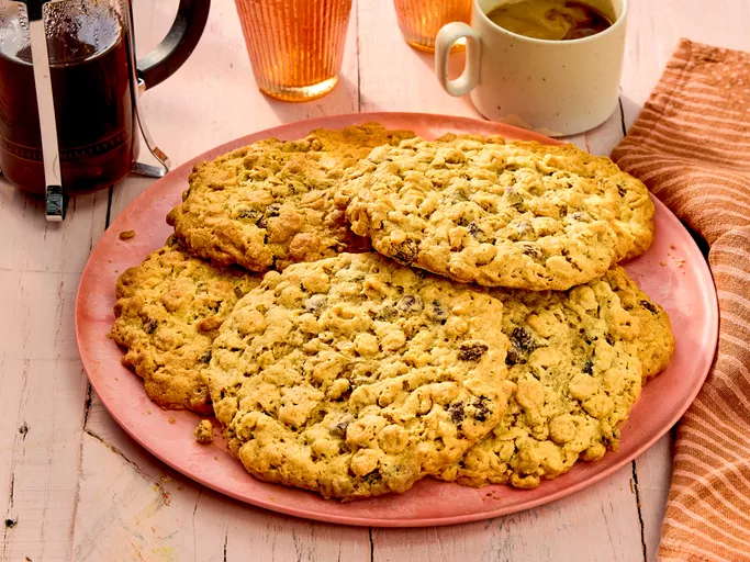
- Enjoy!
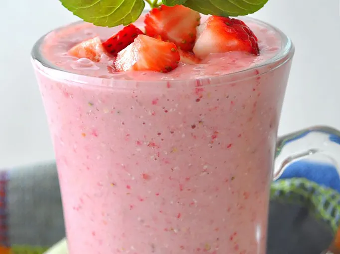
:max_bytes(150000):strip_icc():format(webp)/23539-strawberry-oatmeal-breakfast-smoothie-ddmfs-step-1-0388-9acb7098a2934d5d98a636f96fa3dd27.jpg) Dotdash Meredith Food Studios
Dotdash Meredith Food Studios:max_bytes(150000):strip_icc():format(webp)/23539-strawberry-oatmeal-breakfast-smoothie-ddmfs-step-2-0394-1c0820a02a7b45fc99088ec3c47c044f.jpg)
:max_bytes(150000):strip_icc():format(webp)/23539-strawberry-oatmeal-breakfast-smoothie-ddmfs-step-3-0395-a0559651ddff47688425f37ea19ddc2a.jpg)
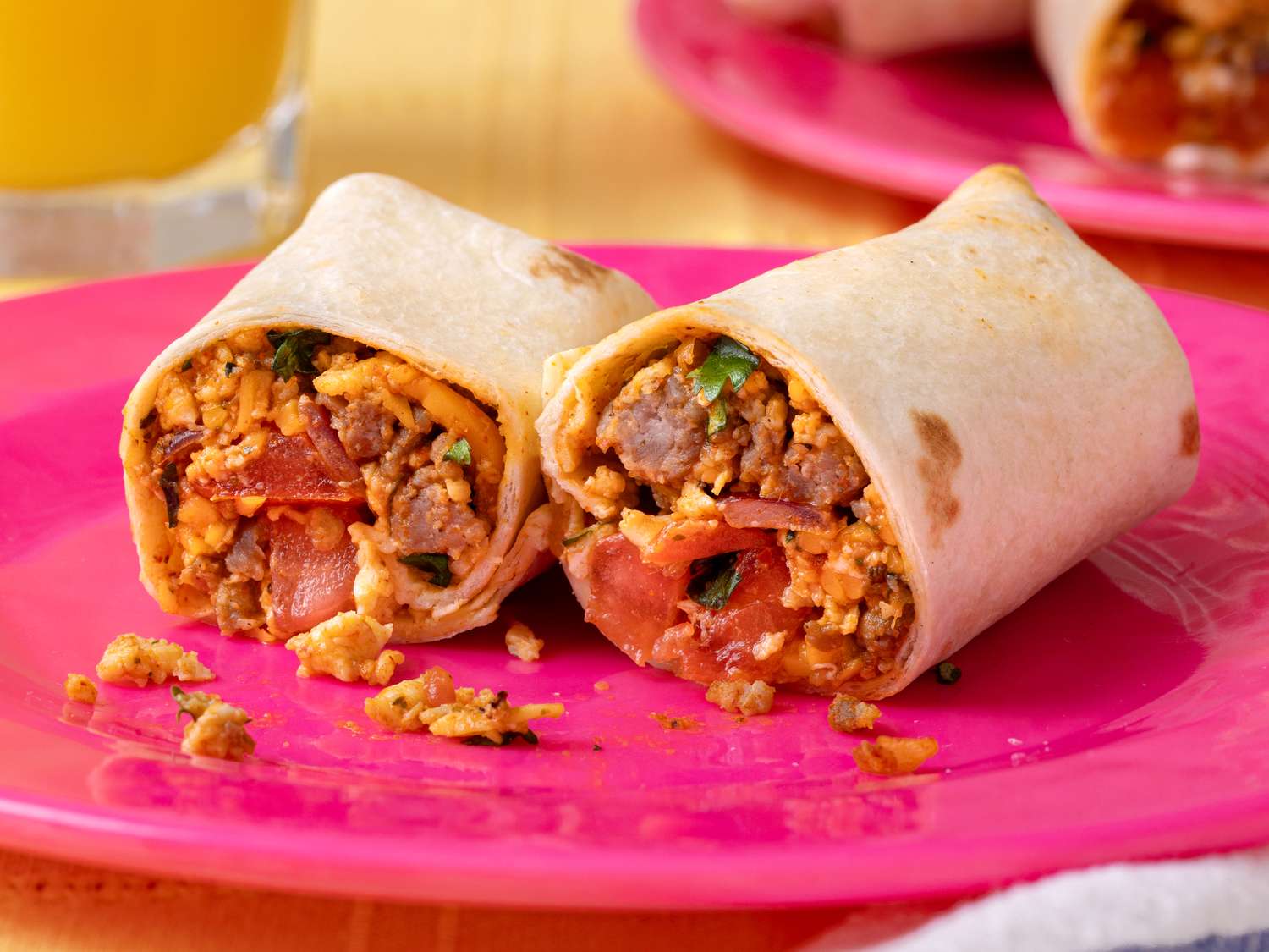
:max_bytes(150000):strip_icc():format(webp)/214583-SouthwestBreakfastBurritos-ddmfs-Step1-3x4-8332-1899aabb978d48a39b541a927f59dd64.jpg) Dotdash Meredith Food Studios
Dotdash Meredith Food Studios:max_bytes(150000):strip_icc():format(webp)/214583-SouthwestBreakfastBurritos-ddmfs-Step2-3x4-8351-f11cd2e06aba45428aa150af23a9870a.jpg) Dotdash Meredith Food Studios
Dotdash Meredith Food Studios:max_bytes(150000):strip_icc():format(webp)/214583-SouthwestBreakfastBurritos-ddmfs-Step3-3x4-8353-83bf6299252244a093d245a2625f87c1.jpg) Dotdash Meredith Food Studios
Dotdash Meredith Food Studios:max_bytes(150000):strip_icc():format(webp)/214583-SouthwestBreakfastBurritos-ddmfs-Step4-3x4-8365-72a695663f114391924636d346c12ed9.jpg) Dotdash Meredith Food Studios
Dotdash Meredith Food Studios:max_bytes(150000):strip_icc():format(webp)/214583-SouthwestBreakfastBurritos-ddmfs-Step6-3x4-8370-f36eea13c04040f2b4e7f74530ed7223.jpg) Dotdash Meredith Food Studios
Dotdash Meredith Food Studios:max_bytes(150000):strip_icc():format(webp)/214583-SouthwestBreakfastBurritos-ddmfs-Step7-3x4-8372-32cd4be21b764c58875b1137ad1b37ba.jpg) Dotdash Meredith Food Studios
Dotdash Meredith Food Studios:max_bytes(150000):strip_icc():format(webp)/214583-SouthwestBreakfastBurritos-ddmfs-Step10-3x4-8378-f48e618d8f674077bc5bc661cc8b6495.jpg) Dotdash Meredith Food Studios
Dotdash Meredith Food Studios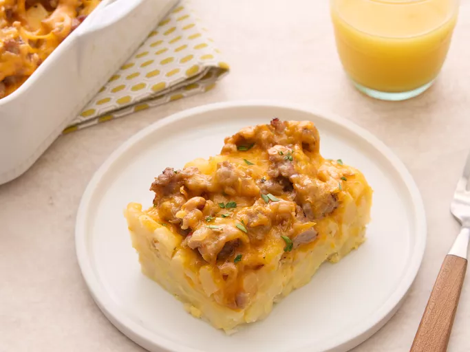
:max_bytes(150000):strip_icc():format(webp)/AR-87013-hash-brown-and-egg-casserole-DDMFS-step-1-a2e320a3175f4433ac18f05630799c67.jpg) Dotdash Meredith Food Studios
Dotdash Meredith Food Studios:max_bytes(150000):strip_icc():format(webp)/AR-87013-hash-brown-and-egg-casserole-DDMFS-step-2-3d6f430003f54adf9a083dbca5201338.jpg) Dotdash Meredith Food Studios
Dotdash Meredith Food Studios:max_bytes(150000):strip_icc():format(webp)/AR-87013-hash-brown-and-egg-casserole-DDMFS-step-4-437a4c39b7e743cfb2c70a0599b48cab.jpg) Dotdash Meredith Food Studios
Dotdash Meredith Food Studios:max_bytes(150000):strip_icc():format(webp)/AR-87013-hash-brown-and-egg-casserole-DDMFS-step-3-e69cf89d792d4e11aa6249290bea0f3b.jpg) Dotdash Meredith Food Studios
Dotdash Meredith Food Studios:max_bytes(150000):strip_icc():format(webp)/AR-87013-hash-brown-and-egg-casserole-DDMFS-step-5-bae8714491fa47f28e138f7f7dc9d7fb.jpg) Dotdash Meredith Food Studios
Dotdash Meredith Food Studios:max_bytes(150000):strip_icc():format(webp)/AR-87013-hash-brown-and-egg-casserole-DDMFS-step-6-353f7c6617e44045ad02397fd323558c.jpg) Dotdash Meredith Food Studios
Dotdash Meredith Food Studios:max_bytes(150000):strip_icc():format(webp)/AR-87013-hash-brown-and-egg-casserole-DDMFS-step-7-7e8b40c5db4644528a2db4d70a79ead5.jpg) Dotdash Meredith Food Studios
Dotdash Meredith Food Studios
:max_bytes(150000):strip_icc():format(webp)/84065-jimmy-dean-breakfast-casserole-ddmfs-step-1-0842-93e0d9f420384bb1a836fc7ecad93ffd.jpg) Dotdash Meredith Food Studios
Dotdash Meredith Food Studios:max_bytes(150000):strip_icc():format(webp)/84065-jimmy-dean-breakfast-casserole-ddmfs-step-2-0845-d2c0abed0d7c4be6ab381b76ebb42d05.jpg) Dotdash Meredith Food Studios
Dotdash Meredith Food Studios:max_bytes(150000):strip_icc():format(webp)/84065-jimmy-dean-breakfast-casserole-ddmfs-step-3-0848-1908292f63f54df28cc569475f5c0999.jpg) Dotdash Meredith Food Studios
Dotdash Meredith Food Studios:max_bytes(150000):strip_icc():format(webp)/84065-jimmy-dean-breakfast-casserole-ddmfs-step-4-0849-99c3377756e5403ea1fb5e5df7f6663d.jpg) Dotdash Meredith Food Studios
Dotdash Meredith Food Studios
:max_bytes(150000):strip_icc():format(webp)/9247-christmas-breakfast-sausage-casserole-step-1-248-df919a8ebdf84a339fc0a59704ccb7eb.jpg) Dotdash Meredith Food Studios
Dotdash Meredith Food Studios:max_bytes(150000):strip_icc():format(webp)/9247-christmas-breakfast-sausage-casserole-step-2-256-949ebf4e99ed4c68a5cba5d43e3a3013.jpg) Dotdash Meredith Food Studios
Dotdash Meredith Food Studios:max_bytes(150000):strip_icc():format(webp)/9247-christmas-breakfast-sausage-casserole-step-3-259-63e824ceb66546ffa765e6acbd18e915.jpg) Dotdash Meredith Food Studios
Dotdash Meredith Food Studios:max_bytes(150000):strip_icc():format(webp)/9247-christmas-breakfast-sausage-casserole-step-4-326-73a88261136d4825856a400e8f75efba.jpg) Dotdash Meredith Food Studios
Dotdash Meredith Food Studios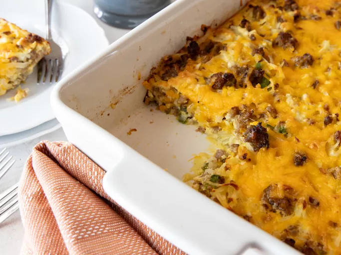
:max_bytes(150000):strip_icc():format(webp)/179351-impossibly-easy-breakfast-bake-crowd-size-VAT-9662-step-01-b01be7c0bb0a4423ab30b72ce6e32a9f.jpg) Allrecipes / Karen Hibbard
Allrecipes / Karen Hibbard:max_bytes(150000):strip_icc():format(webp)/179351-impossibly-easy-breakfast-bake-crowd-size-VAT-9663-step-02-c746cff3d8e94788b857e4e5ec018c64.jpg) Allrecipes / Karen Hibbard
Allrecipes / Karen Hibbard:max_bytes(150000):strip_icc():format(webp)/179351-impossibly-easy-breakfast-bake-crowd-size-VAT-9667-step-03-9a26b158771843459ed1d26f8c4ef586.jpg) Allrecipes / Karen Hibbard
Allrecipes / Karen Hibbard:max_bytes(150000):strip_icc():format(webp)/179351-impossibly-easy-breakfast-bake-crowd-size-VAT-9672-step-04-fde2513067e048fa9690fd6b54c742dc.jpg) Allrecipes / Karen Hibbard
Allrecipes / Karen Hibbard:max_bytes(150000):strip_icc():format(webp)/179351-impossibly-easy-breakfast-bake-crowd-size-VAT-9674-step-05-6c6967465a42481592933888d6dadc66.jpg) Allrecipes / Karen Hibbard
Allrecipes / Karen Hibbard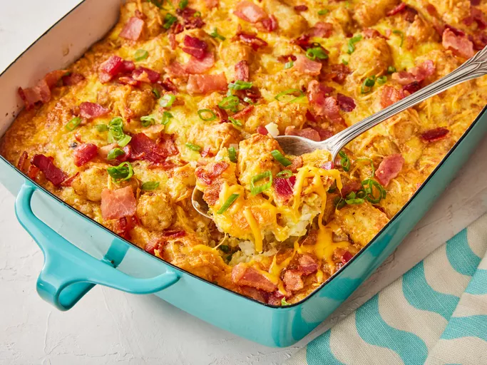
:max_bytes(150000):strip_icc():format(webp)/242266-tater-tot-and-bacon-breakfast-casserole-DDMFS-step-01-0916-2547563ba5524aa19c501dd7b5c61119.jpg) Dotdash Meredith Food Studios
Dotdash Meredith Food Studios:max_bytes(150000):strip_icc():format(webp)/242266-tater-tot-and-bacon-breakfast-casserole-DDMFS-step-01-1-0917-98ac756de9744d939185b81a6506c8ec.jpg) Dotdash Meredith Food Studios
Dotdash Meredith Food Studios:max_bytes(150000):strip_icc():format(webp)/242266-tater-tot-and-bacon-breakfast-casserole-DDMFS-step-02-0919-3fef130fa0934726b88909a29b4c71c9.jpg) Dotdash Meredith Food Studios
Dotdash Meredith Food Studios:max_bytes(150000):strip_icc():format(webp)/242266-tater-tot-and-bacon-breakfast-casserole-DDMFS-step-03-0923-5bcc2506e53643e8a7fe73b3b0d8c6b0.jpg) Dotdash Meredith Food Studios
Dotdash Meredith Food Studios:max_bytes(150000):strip_icc():format(webp)/242266-tater-tot-and-bacon-breakfast-casserole-DDMFS-step-04-0928-1627146496914b56b7d4e703abce0f0d.jpg) Dotdash Meredith Food Studios
Dotdash Meredith Food Studios