Author: saqibkhan

Keras allows to create our own customized layer. Once a new layer is created, it can be used in any model without any restriction. Let us learn how to create new layer in this chapter.

Keras provides a base layer class, Layer which can sub-classed to create our own customized layer. Let us create a simple layer which will find weight based on normal distribution and then do the basic computation of finding the summation of the product of input and its weight during training.

Step 1: Import the necessary module

First, let us import the necessary modules −

from keras import backend as K 
from keras.layers import Layer

Here,

• backend is used to access the dot function.
• Layer is the base class and we will be sub-classing it to create our layer

Step 2: Define a layer class

Let us create a new class, MyCustomLayer by sub-classing Layer class −

class MyCustomLayer(Layer): 
   ...

Step 3: Initialize the layer class

Let us initialize our new class as specified below −

def __init__(self, output_dim, **kwargs):    
   self.output_dim = output_dim 
   super(MyCustomLayer, self).__init__(**kwargs)

Here,

• Line 2 sets the output dimension.
• Line 3 calls the base or super layer’s init function.

Step 4: Implement build method

build is the main method and its only purpose is to build the layer properly. It can do anything related to the inner working of the layer. Once the custom functionality is done, we can call the base class build function. Our custom build function is as follows −

def build(self, input_shape): 
   self.kernel = self.add_weight(name = 'kernel', 
  shape = (input_shape[1], self.output_dim), 
  initializer = 'normal', trainable = True) 
   super(MyCustomLayer, self).build(input_shape)

Here,

• Line 1 defines the build method with one argument, input_shape. Shape of the input data is referred by input_shape.
• Line 2 creates the weight corresponding to input shape and set it in the kernel. It is our custom functionality of the layer. It creates the weight using ‘normal’ initializer.
• Line 6 calls the base class, build method.

Step 5: Implement call method

call method does the exact working of the layer during training process.

Our custom call method is as follows

def call(self, input_data): 
   return K.dot(input_data, self.kernel)

Here,

• Line 1 defines the call method with one argument, input_data. input_data is the input data for our layer.
• Line 2 return the dot product of the input data, input_data and our layer’s kernel, self.kernel

Step 6: Implement compute_output_shape method

def compute_output_shape(self, input_shape): return (input_shape[0], self.output_dim)

Here,

• Line 1 defines compute_output_shape method with one argument input_shape
• Line 2 computes the output shape using shape of input data and output dimension set while initializing the layer.

Implementing the build, call and compute_output_shape completes the creating a customized layer. The final and complete code is as follows

from keras import backend as K from keras.layers import Layer
class MyCustomLayer(Layer): 
   def __init__(self, output_dim, **kwargs): 
  self.output_dim = output_dim 
  super(MyCustomLayer, self).__init__(**kwargs) 
   def build(self, input_shape): self.kernel = 
  self.add_weight(name = 'kernel', 
  shape = (input_shape[1], self.output_dim), 
  initializer = 'normal', trainable = True) 
  super(MyCustomLayer, self).build(input_shape) # 
  Be sure to call this at the end 
   def call(self, input_data): return K.dot(input_data, self.kernel) 
   def compute_output_shape(self, input_shape): return (input_shape[0], self.output_dim)

Using our customized layer

Let us create a simple model using our customized layer as specified below −

from keras.models import Sequential 
from keras.layers import Dense 

model = Sequential() 
model.add(MyCustomLayer(32, input_shape = (16,))) 
model.add(Dense(8, activation = 'softmax')) model.summary()

Here,

• Our MyCustomLayer is added to the model using 32 units and (16,) as input shape

Running the application will print the model summary as below −

Model: "sequential_1" 
_________________________________________________________________ 
Layer (type) Output Shape Param 
#================================================================ 
my_custom_layer_1 (MyCustomL (None, 32) 512 
_________________________________________________________________
dense_1 (Dense) (None, 8) 264 
================================================================= 
Total params: 776 
Trainable params: 776 
Non-trainable params: 0 

As learned earlier, Keras layers are the primary building block of Keras models. Each layer receives input information, do some computation and finally output the transformed information. The output of one layer will flow into the next layer as its input. Let us learn complete details about layers in this chapter.

Introduction

A Keras layer requires shape of the input (input_shape) to understand the structure of the input data, initializer to set the weight for each input and finally activators to transform the output to make it non-linear. In between, constraints restricts and specify the range in which the weight of input data to be generated and regularizer will try to optimize the layer (and the model) by dynamically applying the penalties on the weights during optimization process.

To summarise, Keras layer requires below minimum details to create a complete layer.

• Shape of the input data
• Number of neurons / units in the layer
• Initializers
• Regularizers
• Constraints
• Activations

Let us understand the basic concept in the next chapter. Before understanding the basic concept, let us create a simple Keras layer using Sequential model API to get the idea of how Keras model and layer works.

from keras.models import Sequential 
from keras.layers import Activation, Dense 
from keras import initializers 
from keras import regularizers 
from keras import constraints 

model = Sequential() 

model.add(Dense(32, input_shape=(16,), kernel_initializer = 'he_uniform', 
   kernel_regularizer = None, kernel_constraint = 'MaxNorm', activation = 'relu')) 
model.add(Dense(16, activation = 'relu')) 
model.add(Dense(8))

where,

• Line 1-5 imports the necessary modules.
• Line 7 creates a new model using Sequential API.
• Line 9 creates a new Dense layer and add it into the model. Dense is an entry level layer provided by Keras, which accepts the number of neurons or units (32) as its required parameter. If the layer is first layer, then we need to provide Input Shape, (16,) as well. Otherwise, the output of the previous layer will be used as input of the next layer. All other parameters are optional.
  • First parameter represents the number of units (neurons).
  • input_shape represent the shape of input data.
  • kernel_initializer represent initializer to be used. he_uniform function is set as value.
  • kernel_regularizer represent regularizer to be used. None is set as value.
  • kernel_constraint represent constraint to be used. MaxNorm function is set as value.
  • activation represent activation to be used. relu function is set as value.
• Line 10 creates second Dense layer with 16 units and set relu as the activation function.
• Line 11 creates final Dense layer with 8 units.

Basic Concept of Layers

Let us understand the basic concept of layer as well as how Keras supports each concept.

Input shape

In machine learning, all type of input data like text, images or videos will be first converted into array of numbers and then feed into the algorithm. Input numbers may be single dimensional array, two dimensional array (matrix) or multi-dimensional array. We can specify the dimensional information using shape, a tuple of integers. For example, (4,2) represent matrix with four rows and two columns.

>>> import numpy as np 
>>> shape = (4, 2) 
>>> input = np.zeros(shape) 
>>> print(input) 
[
   [0. 0.] 
   [0. 0.] 
   [0. 0.] 
   [0. 0.]
] 
>>>

Similarly, (3,4,2) three dimensional matrix having three collections of 4×2 matrix (two rows and four columns).

>>> import numpy as np 
>>> shape = (3, 4, 2) 
>>> input = np.zeros(shape) 
>>> print(input)
[
   [[0. 0.] [0. 0.] [0. 0.] [0. 0.]] 
   [[0. 0.] [0. 0.] [0. 0.] [0. 0.]] 
   [[0. 0.] [0. 0.] [0. 0.] [0. 0.]]
]
>>>

To create the first layer of the model (or input layer of the model), shape of the input data should be specified.

Explore our latest online courses and learn new skills at your own pace. Enroll and become a certified expert to boost your career.

Initializers

In Machine Learning, weight will be assigned to all input data. Initializers module provides different functions to set these initial weight. Some of the Keras Initializer function are as follows −

Zeros

Generates 0 for all input data.

from keras.models import Sequential 
from keras.layers import Activation, Dense 
from keras import initializers 

my_init = initializers.Zeros() 
model = Sequential() 
model.add(Dense(512, activation = 'relu', input_shape = (784,), 
   kernel_initializer = my_init))

Where, kernel_initializer represent the initializer for kernel of the model.

Ones

Generates 1 for all input data.

from keras.models import Sequential 
from keras.layers import Activation, Dense 
from keras import initializers 

my_init = initializers.Ones() 
model.add(Dense(512, activation = 'relu', input_shape = (784,), 
   kernel_initializer = my_init))

Constant

Generates a constant value (say, 5) specified by the user for all input data.

from keras.models import Sequential 
from keras.layers import Activation, Dense 
from keras import initializers 

my_init = initializers.Constant(value = 0) model.add(
   Dense(512, activation = 'relu', input_shape = (784,), kernel_initializer = my_init)
)

where, value represent the constant value

RandomNormal

Generates value using normal distribution of input data.

from keras.models import Sequential 
from keras.layers import Activation, Dense 
from keras import initializers 

my_init = initializers.RandomNormal(mean=0.0, 
stddev = 0.05, seed = None) 
model.add(Dense(512, activation = 'relu', input_shape = (784,), 
   kernel_initializer = my_init))

where,

• mean represent the mean of the random values to generate
• stddev represent the standard deviation of the random values to generate
• seed represent the values to generate random number

RandomUniform

Generates value using uniform distribution of input data.

from keras import initializers 

my_init = initializers.RandomUniform(minval = -0.05, maxval = 0.05, seed = None) 
model.add(Dense(512, activation = 'relu', input_shape = (784,), 
   kernel_initializer = my_init))

where,

• minval represent the lower bound of the random values to generate
• maxval represent the upper bound of the random values to generate

TruncatedNormal

Generates value using truncated normal distribution of input data.

from keras.models import Sequential 
from keras.layers import Activation, Dense 
from keras import initializers 

my_init = initializers.TruncatedNormal(mean = 0.0, stddev = 0.05, seed = None
model.add(Dense(512, activation = 'relu', input_shape = (784,), 
   kernel_initializer = my_init))

VarianceScaling

Generates value based on the input shape and output shape of the layer along with the specified scale.

from keras.models import Sequential 
from keras.layers import Activation, Dense 
from keras import initializers 

my_init = initializers.VarianceScaling(
   scale = 1.0, mode = 'fan_in', distribution = 'normal', seed = None) 
model.add(Dense(512, activation = 'relu', input_shape = (784,), 
   skernel_initializer = my_init))

where,

• scale represent the scaling factor
• mode represent any one of fan_in, fan_out and fan_avg values
• distribution represent either of normal or uniform

VarianceScaling

It finds the stddev value for normal distribution using below formula and then find the weights using normal distribution,

stddev = sqrt(scale / n)

where n represent,

• number of input units for mode = fan_in
• number of out units for mode = fan_out
• average number of input and output units for mode = fan_avg

Similarly, it finds the limit for uniform distribution using below formula and then find the weights using uniform distribution,

limit = sqrt(3 * scale / n)

lecun_normal

Generates value using lecun normal distribution of input data.

from keras.models import Sequential 
from keras.layers import Activation, Dense 
from keras import initializers 

my_init = initializers.RandomUniform(minval = -0.05, maxval = 0.05, seed = None)
model.add(Dense(512, activation = 'relu', input_shape = (784,), 
   kernel_initializer = my_init))

It finds the stddev using the below formula and then apply normal distribution

stddev = sqrt(1 / fan_in)

where, fan_in represent the number of input units.

lecun_uniform

Generates value using lecun uniform distribution of input data.

from keras.models import Sequential 
from keras.layers import Activation, Dense 
from keras import initializers 

my_init = initializers.lecun_uniform(seed = None) 
model.add(Dense(512, activation = 'relu', input_shape = (784,), 
   kernel_initializer = my_init))

It finds the limit using the below formula and then apply uniform distribution

limit = sqrt(3 / fan_in)

where,

• fan_in represents the number of input units
• fan_out represents the number of output units

glorot_normal

Generates value using glorot normal distribution of input data.

from keras.models import Sequential 
from keras.layers import Activation, Dense 
from keras import initializers 

my_init = initializers.glorot_normal(seed=None) model.add(
   Dense(512, activation = 'relu', input_shape = (784,), kernel_initializer = my_init)
)

It finds the stddev using the below formula and then apply normal distribution

stddev = sqrt(2 / (fan_in + fan_out))

where,

• fan_in represents the number of input units
• fan_out represents the number of output units

glorot_uniform

Generates value using glorot uniform distribution of input data.

from keras.models import Sequential 
from keras.layers import Activation, Dense 
from keras import initializers 

my_init = initializers.glorot_uniform(seed = None) 
model.add(Dense(512, activation = 'relu', input_shape = (784,), 
   kernel_initializer = my_init))

It finds the limit using the below formula and then apply uniform distribution

limit = sqrt(6 / (fan_in + fan_out))

where,

• fan_in represent the number of input units.
• fan_out represents the number of output units

he_normal

Generates value using he normal distribution of input data.

from keras.models import Sequential 
from keras.layers import Activation, Dense 
from keras import initializers 

my_init = initializers.RandomUniform(minval = -0.05, maxval = 0.05, seed = None) 
model.add(Dense(512, activation = 'relu', input_shape = (784,), 
   kernel_initializer = my_init))

It finds the stddev using the below formula and then apply normal distribution.

stddev = sqrt(2 / fan_in)

where, fan_in represent the number of input units.

he_uniform

Generates value using he uniform distribution of input data.

from keras.models import Sequential 
from keras.layers import Activation, Dense 
from keras import initializers 

my_init = initializers.he_normal(seed = None) 
model.add(Dense(512, activation = 'relu', input_shape = (784,), 
   kernel_initializer = my_init))

It finds the limit using the below formula and then apply uniform distribution.

limit = sqrt(6 / fan_in)

where, fan_in represent the number of input units.

Orthogonal

Generates a random orthogonal matrix.

from keras.models import Sequential 
from keras.layers import Activation, Dense 
from keras import initializers 

my_init = initializers.Orthogonal(gain = 1.0, seed = None) 
model.add(Dense(512, activation = 'relu', input_shape = (784,), 
   kernel_initializer = my_init))

where, gain represent the multiplication factor of the matrix.

Identity

Generates identity matrix.

from keras.models import Sequential 
from keras.layers import Activation, Dense 
from keras import initializers 

my_init = initializers.Identity(gain = 1.0) model.add(
   Dense(512, activation = 'relu', input_shape = (784,), kernel_initializer = my_init)
)

Constraints

In machine learning, a constraint will be set on the parameter (weight) during optimization phase. <>Constraints module provides different functions to set the constraint on the layer. Some of the constraint functions are as follows.

NonNeg

Constrains weights to be non-negative.

from keras.models import Sequential 
from keras.layers import Activation, Dense 
from keras import initializers 

my_init = initializers.Identity(gain = 1.0) model.add(
   Dense(512, activation = 'relu', input_shape = (784,), 
   kernel_initializer = my_init)
)

where, kernel_constraint represent the constraint to be used in the layer.

UnitNorm

Constrains weights to be unit norm.

from keras.models import Sequential 
from keras.layers import Activation, Dense 
from keras import constraints 

my_constrain = constraints.UnitNorm(axis = 0) 
model = Sequential() 
model.add(Dense(512, activation = 'relu', input_shape = (784,), 
   kernel_constraint = my_constrain))

MaxNorm

Constrains weight to norm less than or equals to the given value.

from keras.models import Sequential 
from keras.layers import Activation, Dense 
from keras import constraints 

my_constrain = constraints.MaxNorm(max_value = 2, axis = 0) 
model = Sequential() 
model.add(Dense(512, activation = 'relu', input_shape = (784,), 
   kernel_constraint = my_constrain))

where,

• max_value represent the upper bound
• axis represent the dimension in which the constraint to be applied. e.g. in Shape (2,3,4) axis 0 denotes first dimension, 1 denotes second dimension and 2 denotes third dimension

MinMaxNorm

Constrains weights to be norm between specified minimum and maximum values.

from keras.models import Sequential 
from keras.layers import Activation, Dense 
from keras import constraints 

my_constrain = constraints.MinMaxNorm(min_value = 0.0, max_value = 1.0, rate = 1.0, axis = 0) 
model = Sequential() 
model.add(Dense(512, activation = 'relu', input_shape = (784,), 
   kernel_constraint = my_constrain))

where, rate represent the rate at which the weight constrain is applied.

Regularizers

In machine learning, regularizers are used in the optimization phase. It applies some penalties on the layer parameter during optimization. Keras regularization module provides below functions to set penalties on the layer. Regularization applies per-layer basis only.

L1 Regularizer

It provides L1 based regularization.

from keras.models import Sequential 
from keras.layers import Activation, Dense 
from keras import regularizers 

my_regularizer = regularizers.l1(0.) 
model = Sequential() 
model.add(Dense(512, activation = 'relu', input_shape = (784,), 
   kernel_regularizer = my_regularizer))

where, kernel_regularizer represent the rate at which the weight constrain is applied.

L2 Regularizer

It provides L2 based regularization.

from keras.models import Sequential 
from keras.layers import Activation, Dense 
from keras import regularizers 

my_regularizer = regularizers.l2(0.) 
model = Sequential() 
model.add(Dense(512, activation = 'relu', input_shape = (784,), 
   kernel_regularizer = my_regularizer))

L1 and L2 Regularizer

It provides both L1 and L2 based regularization.

from keras.models import Sequential 
from keras.layers import Activation, Dense 
from keras import regularizers 

my_regularizer = regularizers.l2(0.) 
model = Sequential() 
model.add(Dense(512, activation = 'relu', input_shape = (784,),
   kernel_regularizer = my_regularizer))

Activations

In machine learning, activation function is a special function used to find whether a specific neuron is activated or not. Basically, the activation function does a nonlinear transformation of the input data and thus enable the neurons to learn better. Output of a neuron depends on the activation function.

As you recall the concept of single perception, the output of a perceptron (neuron) is simply the result of the activation function, which accepts the summation of all input multiplied with its corresponding weight plus overall bias, if any available.

result = Activation(SUMOF(input * weight) + bias)

So, activation function plays an important role in the successful learning of the model. Keras provides a lot of activation function in the activations module. Let us learn all the activations available in the module.

linear

Applies Linear function. Does nothing.

from keras.models import Sequential 
from keras.layers import Activation, Dense 

model = Sequential() 
model.add(Dense(512, activation = 'linear', input_shape = (784,)))

Where, activation refers the activation function of the layer. It can be specified simply by the name of the function and the layer will use corresponding activators.

elu

Applies Exponential linear unit.

from keras.models import Sequential 
from keras.layers import Activation, Dense 

model = Sequential() 
model.add(Dense(512, activation = 'elu', input_shape = (784,)))

selu

Applies Scaled exponential linear unit.

from keras.models import Sequential 
from keras.layers import Activation, Dense 

model = Sequential() 
model.add(Dense(512, activation = 'selu', input_shape = (784,)))

relu

Applies Rectified Linear Unit.

from keras.models import Sequential 
from keras.layers import Activation, Dense 

model = Sequential() 
model.add(Dense(512, activation = 'relu', input_shape = (784,)))

softmax

Applies Softmax function.

from keras.models import Sequential 
from keras.layers import Activation, Dense 

model = Sequential() 
model.add(Dense(512, activation = 'softmax', input_shape = (784,)))

softplus

Applies Softplus function.

from keras.models import Sequential 
from keras.layers import Activation, Dense 

model = Sequential() 
model.add(Dense(512, activation = 'softplus', input_shape = (784,)))

softsign

Applies Softsign function.

from keras.models import Sequential 
from keras.layers import Activation, Dense 

model = Sequential() 
model.add(Dense(512, activation = 'softsign', input_shape = (784,)))

tanh

Applies Hyperbolic tangent function.

from keras.models import Sequential 
from keras.layers import Activation, Dense 
model = Sequential() 
model.add(Dense(512, activation = 'tanh', input_shape = (784,)))

sigmoid

Applies Sigmoid function.

from keras.models import Sequential 
from keras.layers import Activation, Dense 

model = Sequential() 
model.add(Dense(512, activation = 'sigmoid', input_shape = (784,)))

hard_sigmoid

Applies Hard Sigmoid function.

from keras.models import Sequential 
from keras.layers import Activation, Dense 

model = Sequential() 
model.add(Dense(512, activation = 'hard_sigmoid', input_shape = (784,)))

exponential

Applies exponential function.

from keras.models import Sequential 
from keras.layers import Activation, Dense 

model = Sequential() 
model.add(Dense(512, activation = 'exponential', input_shape = (784,)))

Sr.No	Layers & Description
1	Dense LayerDense layer is the regular deeply connected neural network layer.
2	Dropout LayersDropout is one of the important concept in the machine learning.
3	Flatten LayersFlatten is used to flatten the input.
4	Reshape LayersReshape is used to change the shape of the input.
5	Permute LayersPermute is also used to change the shape of the input using pattern.
6	RepeatVector LayersRepeatVector is used to repeat the input for set number, n of times.
7	Lambda LayersLambda is used to transform the input data using an expression or function.
8	Convolution LayersKeras contains a lot of layers for creating Convolution based ANN, popularly called as Convolution Neural Network (CNN).
9	Pooling LayerIt is used to perform max pooling operations on temporal data.
10	Locally connected layerLocally connected layers are similar to Conv1D layer but the difference is Conv1D layer weights are shared but here weights are unshared.
11	Merge LayerIt is used to merge a list of inputs.
12	Embedding LayerIt performs embedding operations in input layer.

As we learned earlier, Keras modules contains pre-defined classes, functions and variables which are useful for deep learning algorithm. Let us learn the modules provided by Keras in this chapter.

Available modules

Let us first see the list of modules available in the Keras.

• Initializers − Provides a list of initializers function. We can learn it in details in Keras layer chapter. during model creation phase of machine learning.
• Regularizers − Provides a list of regularizers function. We can learn it in details in Keras Layers chapter.
• Constraints − Provides a list of constraints function. We can learn it in details in Keras Layers chapter.
• Activations − Provides a list of activator function. We can learn it in details in Keras Layers chapter.
• Losses − Provides a list of loss function. We can learn it in details in Model Training chapter.
• Metrics − Provides a list of metrics function. We can learn it in details in Model Training chapter.
• Optimizers − Provides a list of optimizer function. We can learn it in details in Model Training chapter.
• Callback − Provides a list of callback function. We can use it during the training process to print the intermediate data as well as to stop the training itself (EarlyStopping method) based on some condition.
• Text processing − Provides functions to convert text into NumPy array suitable for machine learning. We can use it in data preparation phase of machine learning.
• Image processing − Provides functions to convert images into NumPy array suitable for machine learning. We can use it in data preparation phase of machine learning.
• Sequence processing − Provides functions to generate time based data from the given input data. We can use it in data preparation phase of machine learning.
• Backend − Provides function of the backend library like TensorFlow and Theano.
• Utilities − Provides lot of utility function useful in deep learning.

Let us see backend module and utils model in this chapter.

backend module

backend module is used for keras backend operations. By default, keras runs on top of TensorFlow backend. If you want, you can switch to other backends like Theano or CNTK. Defualt backend configuration is defined inside your root directory under .keras/keras.json file.

Keras backend module can be imported using below code

>>> from keras import backend as k

If we are using default backend TensorFlow, then the below function returns TensorFlow based information as specified below −

>>> k.backend() 
'tensorflow'
>>> k.epsilon() 
1e-07
>>> k.image_data_format() 
'channels_last'
>>> k.floatx() 
'float32'

Let us understand some of the significant backend functions used for data analysis in brief −

get_uid()

It is the identifier for the default graph. It is defined below −

>>> k.get_uid(prefix='') 
1 
>>> k.get_uid(prefix='') 2

reset_uids

It is used resets the uid value.

>>> k.reset_uids()

Now, again execute the get_uid(). This will be reset and change again to 1.

>>> k.get_uid(prefix='') 
1

placeholder

It is used instantiates a placeholder tensor. Simple placeholder to hold 3-D shape is shown below −

>>> data = k.placeholder(shape = (1,3,3)) 
>>> data 
<tf.Tensor 'Placeholder_9:0' shape = (1, 3, 3) dtype = float32> 

If you use int_shape(), it will show the shape. 

>>> k.int_shape(data) (1, 3, 3)

dot

It is used to multiply two tensors. Consider a and b are two tensors and c will be the outcome of multiply of ab. Assume a shape is (4,2) and b shape is (2,3). It is defined below,

>>> a = k.placeholder(shape = (4,2)) 
>>> b = k.placeholder(shape = (2,3)) 
>>> c = k.dot(a,b) 
>>> c 
<tf.Tensor 'MatMul_3:0' shape = (4, 3) dtype = float32> 
>>>

ones

It is used to initialize all as one value.

>>> res = k.ones(shape = (2,2)) 

#print the value 

>>> k.eval(res) 
array([[1., 1.], [1., 1.]], dtype = float32)

batch_dot

It is used to perform the product of two data in batches. Input dimension must be 2 or higher. It is shown below −

>>> a_batch = k.ones(shape = (2,3)) 
>>> b_batch = k.ones(shape = (3,2)) 
>>> c_batch = k.batch_dot(a_batch,b_batch) 
>>> c_batch 
<tf.Tensor 'ExpandDims:0' shape = (2, 1) dtype = float32>

variable

It is used to initializes a variable. Let us perform simple transpose operation in this variable.

>>> data = k.variable([[10,20,30,40],[50,60,70,80]]) 
#variable initialized here 
>>> result = k.transpose(data) 
>>> print(result) 
Tensor("transpose_6:0", shape = (4, 2), dtype = float32) 
>>> print(k.eval(result)) 
   [[10. 50.] 
   [20. 60.] 
   [30. 70.] 
   [40. 80.]]

If you want to access from numpy −

>>> data = np.array([[10,20,30,40],[50,60,70,80]]) 

>>> print(np.transpose(data)) 
   [[10 50] 
   [20 60] 
   [30 70] 
   [40 80]] 

>>> res = k.variable(value = data) 
>>> print(res) 
<tf.Variable 'Variable_7:0' shape = (2, 4) dtype = float32_ref>

is_sparse(tensor)

It is used to check whether the tensor is sparse or not.

>>> a = k.placeholder((2, 2), sparse=True) 

>>> print(a) SparseTensor(indices =       
   Tensor("Placeholder_8:0", 
   shape = (?, 2), dtype = int64), 
values = Tensor("Placeholder_7:0", shape = (?,), 
dtype = float32), dense_shape = Tensor("Const:0", shape = (2,), dtype = int64)) 

>>> print(k.is_sparse(a)) True

to_dense()

It is used to converts sparse into dense.

>>> b = k.to_dense(a) 
>>> print(b) Tensor("SparseToDense:0", shape = (2, 2), dtype = float32) 
>>> print(k.is_sparse(b)) False

random_uniform_variable

It is used to initialize using uniform distribution concept.

k.random_uniform_variable(shape, mean, scale)

Here,

• shape − denotes the rows and columns in the format of tuples.
• mean − mean of uniform distribution.
• scale − standard deviation of uniform distribution.

Let us have a look at the below example usage −

>>> a = k.random_uniform_variable(shape = (2, 3), low=0, high = 1) 
>>> b = k. random_uniform_variable(shape = (3,2), low = 0, high = 1) 
>>> c = k.dot(a, b) 
>>> k.int_shape(c) 
(2, 2)

Explore our latest online courses and learn new skills at your own pace. Enroll and become a certified expert to boost your career.

utils module

utils provides useful utilities function for deep learning. Some of the methods provided by the utils module is as follows −

HDF5Matrix

It is used to represent the input data in HDF5 format.

from keras.utils import HDF5Matrix data = HDF5Matrix('data.hdf5', 'data')

to_categorical

It is used to convert class vector into binary class matrix.

>>> from keras.utils import to_categorical 
>>> labels = [0, 1, 2, 3, 4, 5, 6, 7, 8, 9] 
>>> to_categorical(labels) 
array([[1., 0., 0., 0., 0., 0., 0., 0., 0., 0.], 
   [0., 1., 0., 0., 0., 0., 0., 0., 0., 0.], 
   [0., 0., 1., 0., 0., 0., 0., 0., 0., 0.], 
   [0., 0., 0., 1., 0., 0., 0., 0., 0., 0.], 
   [0., 0., 0., 0., 1., 0., 0., 0., 0., 0.], 
   [0., 0., 0., 0., 0., 1., 0., 0., 0., 0.], 
   [0., 0., 0., 0., 0., 0., 1., 0., 0., 0.], 
   [0., 0., 0., 0., 0., 0., 0., 1., 0., 0.], 
   [0., 0., 0., 0., 0., 0., 0., 0., 1., 0.], 
   [0., 0., 0., 0., 0., 0., 0., 0., 0., 1.]], dtype = float32)
>>> from keras.utils import normalize 
>>> normalize([1, 2, 3, 4, 5]) 
array([[0.13483997, 0.26967994, 0.40451992, 0.53935989, 0.67419986]])

print_summary

It is used to print the summary of the model.

from keras.utils import print_summary print_summary(model)

plot_model

It is used to create the model representation in dot format and save it to file.

from keras.utils import plot_model 
plot_model(model,to_file = 'image.png')

This plot_model will generate an image to understand the performance of model.

Keras provides a complete framework to create any type of neural networks. Keras is innovative as well as very easy to learn. It supports simple neural network to very large and complex neural network model. Let us understand the architecture of Keras framework and how Keras helps in deep learning in this chapter.

Architecture of Keras

Keras API can be divided into three main categories −

• Model
• Layer
• Core Modules

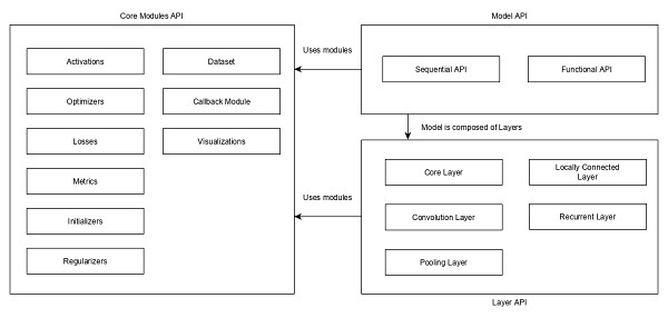
In Keras, every ANN is represented by Keras Models. In turn, every Keras Model is composition of Keras Layers and represents ANN layers like input, hidden layer, output layers, convolution layer, pooling layer, etc., Keras model and layer access Keras modules for activation function, loss function, regularization function, etc., Using Keras model, Keras Layer, and Keras modules, any ANN algorithm (CNN, RNN, etc.,) can be represented in a simple and efficient manner.

The following diagram depicts the relationship between model, layer and core modules −

Let us see the overview of Keras models, Keras layers and Keras modules.

Model

Keras Models are of two types as mentioned below −

Sequential Model − Sequential model is basically a linear composition of Keras Layers. Sequential model is easy, minimal as well as has the ability to represent nearly all available neural networks.

A simple sequential model is as follows −

from keras.models import Sequential 
from keras.layers import Dense, Activation 

model = Sequential()  
model.add(Dense(512, activation = 'relu', input_shape = (784,)))

Where,

• Line 1 imports Sequential model from Keras models
• Line 2 imports Dense layer and Activation module
• Line 4 create a new sequential model using Sequential API
• Line 5 adds a dense layer (Dense API) with relu activation (using Activation module) function.

Sequential model exposes Model class to create customized models as well. We can use sub-classing concept to create our own complex model.

Functional API − Functional API is basically used to create complex models.

Explore our latest online courses and learn new skills at your own pace. Enroll and become a certified expert to boost your career.

Layer

Each Keras layer in the Keras model represent the corresponding layer (input layer, hidden layer and output layer) in the actual proposed neural network model. Keras provides a lot of pre-build layers so that any complex neural network can be easily created. Some of the important Keras layers are specified below,

• Core Layers
• Convolution Layers
• Pooling Layers
• Recurrent Layers

A simple python code to represent a neural network model using sequential model is as follows −

from keras.models import Sequential 
from keras.layers import Dense, Activation, Dropout model = Sequential() 

model.add(Dense(512, activation = 'relu', input_shape = (784,))) 
model.add(Dropout(0.2)) 
model.add(Dense(512, activation = 'relu')) model.add(Dropout(0.2)) 
model.add(Dense(num_classes, activation = 'softmax'))

Where,

• Line 1 imports Sequential model from Keras models
• Line 2 imports Dense layer and Activation module
• Line 4 create a new sequential model using Sequential API
• Line 5 adds a dense layer (Dense API) with relu activation (using Activation module) function.
• Line 6 adds a dropout layer (Dropout API) to handle over-fitting.
• Line 7 adds another dense layer (Dense API) with relu activation (using Activation module) function.
• Line 8 adds another dropout layer (Dropout API) to handle over-fitting.
• Line 9 adds final dense layer (Dense API) with softmax activation (using Activation module) function.

Keras also provides options to create our own customized layers. Customized layer can be created by sub-classing the Keras.Layer class and it is similar to sub-classing Keras models.

Core Modules

Keras also provides a lot of built-in neural network related functions to properly create the Keras model and Keras layers. Some of the function are as follows −

• Activations module − Activation function is an important concept in ANN and activation modules provides many activation function like softmax, relu, etc.,
• Loss module − Loss module provides loss functions like mean_squared_error, mean_absolute_error, poisson, etc.,
• Optimizer module − Optimizer module provides optimizer function like adam, sgd, etc.,
• Regularizers − Regularizer module provides functions like L1 regularizer, L2 regularizer, etc.,

Let us learn Keras modules in detail in the upcoming chapter.

Deep learning is an evolving subfield of machine learning. Deep learning involves analyzing the input in layer by layer manner, where each layer progressively extracts higher level information about the input.

Let us take a simple scenario of analyzing an image. Let us assume that your input image is divided up into a rectangular grid of pixels. Now, the first layer abstracts the pixels. The second layer understands the edges in the image. The Next layer constructs nodes from the edges. Then, the next would find branches from the nodes. Finally, the output layer will detect the full object. Here, the feature extraction process goes from the output of one layer into the input of the next subsequent layer.

By using this approach, we can process huge amount of features, which makes deep learning a very powerful tool. Deep learning algorithms are also useful for the analysis of unstructured data. Let us go through the basics of deep learning in this chapter.

Artificial Neural Networks

The most popular and primary approach of deep learning is using “Artificial neural network” (ANN). They are inspired from the model of human brain, which is the most complex organ of our body. The human brain is made up of more than 90 billion tiny cells called “Neurons”. Neurons are inter-connected through nerve fiber called “axons” and “Dendrites”. The main role of axon is to transmit information from one neuron to another to which it is connected.

Similarly, the main role of dendrites is to receive the information being transmitted by the axons of another neuron to which it is connected. Each neuron processes a small information and then passes the result to another neuron and this process continues. This is the basic method used by our human brain to process huge about of information like speech, visual, etc., and extract useful information from it.

Based on this model, the first Artificial Neural Network (ANN) was invented by psychologist Frank Rosenblatt, in the year of 1958. ANNs are made up of multiple nodes which is similar to neurons. Nodes are tightly interconnected and organized into different hidden layers. The input layer receives the input data and the data goes through one or more hidden layers sequentially and finally the output layer predict something useful about the input data. For example, the input may be an image and the output may be the thing identified in the image, say a “Cat”.

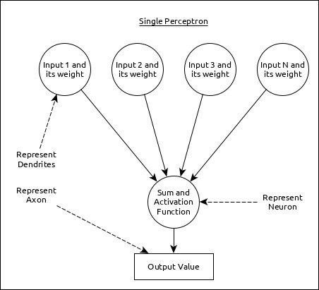
A single neuron (called as perceptron in ANN) can be represented as below −

Here,

• Multiple input along with weight represents dendrites.
• Sum of input along with activation function represents neurons. Sum actually means computed value of all inputs and activation function represent a function, which modify the Sum value into 0, 1 or 0 to 1.
• Actual output represent axon and the output will be received by neuron in next layer.

Let us understand different types of artificial neural networks in this section.

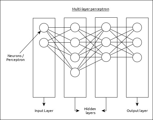
Multi-Layer Perceptron

Multi-Layer perceptron is the simplest form of ANN. It consists of a single input layer, one or more hidden layer and finally an output layer. A layer consists of a collection of perceptron. Input layer is basically one or more features of the input data. Every hidden layer consists of one or more neurons and process certain aspect of the feature and send the processed information into the next hidden layer. The output layer process receives the data from last hidden layer and finally output the result.

Explore our latest online courses and learn new skills at your own pace. Enroll and become a certified expert to boost your career.

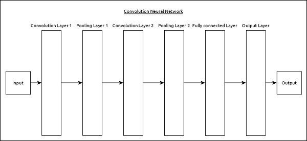
Convolutional Neural Network (CNN)

Convolutional neural network is one of the most popular ANN. It is widely used in the fields of image and video recognition. It is based on the concept of convolution, a mathematical concept. It is almost similar to multi-layer perceptron except it contains series of convolution layer and pooling layer before the fully connected hidden neuron layer. It has three important layers −

• Convolution layer − It is the primary building block and perform computational tasks based on convolution function.
• Pooling layer − It is arranged next to convolution layer and is used to reduce the size of inputs by removing unnecessary information so computation can be performed faster.
• Fully connected layer − It is arranged to next to series of convolution and pooling layer and classify input into various categories.

A simple CNN can be represented as below −

Here,

• 2 series of Convolution and pooling layer is used and it receives and process the input (e.g. image).
• A single fully connected layer is used and it is used to output the data (e.g. classification of image)

Recurrent Neural Network (RNN)

Recurrent Neural Networks (RNN) are useful to address the flaw in other ANN models. Well, Most of the ANN doesn’t remember the steps from previous situations and learned to make decisions based on context in training. Meanwhile, RNN stores the past information and all its decisions are taken from what it has learnt from the past.

This approach is mainly useful in image classification. Sometimes, we may need to look into the future to fix the past. In this case bidirectional RNN is helpful to learn from the past and predict the future. For example, we have handwritten samples in multiple inputs. Suppose, we have confusion in one input then we need to check again other inputs to recognize the correct context which takes the decision from the past.

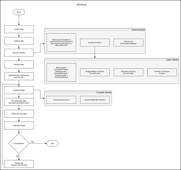
Workflow of ANN

Let us first understand the different phases of deep learning and then, learn how Keras helps in the process of deep learning.

Collect required data

Deep learning requires lot of input data to successfully learn and predict the result. So, first collect as much data as possible.

Analyze data

Analyze the data and acquire a good understanding of the data. The better understanding of the data is required to select the correct ANN algorithm.

Choose an algorithm (model)

Choose an algorithm, which will best fit for the type of learning process (e.g image classification, text processing, etc.,) and the available input data. Algorithm is represented by Model in Keras. Algorithm includes one or more layers. Each layers in ANN can be represented by Keras Layer in Keras.

• Prepare data − Process, filter and select only the required information from the data.
• Split data − Split the data into training and test data set. Test data will be used to evaluate the prediction of the algorithm / Model (once the machine learn) and to cross check the efficiency of the learning process.
• Compile the model − Compile the algorithm / model, so that, it can be used further to learn by training and finally do to prediction. This step requires us to choose loss function and Optimizer. loss function and Optimizer are used in learning phase to find the error (deviation from actual output) and do optimization so that the error will be minimized.
• Fit the model − The actual learning process will be done in this phase using the training data set.
• Predict result for unknown value − Predict the output for the unknown input data (other than existing training and test data)
• Evaluate model − Evaluate the model by predicting the output for test data and cross-comparing the prediction with actual result of the test data.
• Freeze, Modify or choose new algorithm − Check whether the evaluation of the model is successful. If yes, save the algorithm for future prediction purpose. If not, then modify or choose new algorithm / model and finally, again train, predict and evaluate the model. Repeat the process until the best algorithm (model) is found.

The above steps can be represented using below flow chart −

This chapter explains Keras backend implementations TensorFlow and Theano in detail. Let us go through each implementation one by one.

TensorFlow

TensorFlow is an open source machine learning library used for numerical computational tasks developed by Google. Keras is a high level API built on top of TensorFlow or Theano. We know already how to install TensorFlow using pip.

If it is not installed, you can install using the below command −

pip install TensorFlow

Once we execute keras, we could see the configuration file is located at your home directory inside and go to .keras/keras.json.

keras.json

{ 
   "image_data_format": "channels_last", 
   "epsilon": 1e-07, "floatx": "float32", "backend": "tensorflow" 
}

Here,

• image_data_format represent the data format.
• epsilon represents numeric constant. It is used to avoid DivideByZero error.
• floatx represent the default data type float32. You can also change it to float16 or float64 using set_floatx() method.
• image_data_format represent the data format.

Suppose, if the file is not created then move to the location and create using the below steps −

> cd home 
> mkdir .keras 
> vi keras.json

Remember, you should specify .keras as its folder name and add the above configuration inside keras.json file. We can perform some pre-defined operations to know backend functions.

Theano

Theano is an open source deep learning library that allows you to evaluate multi-dimensional arrays effectively. We can easily install using the below command −

pip install theano

By default, keras uses TensorFlow backend. If you want to change backend configuration from TensorFlow to Theano, just change the backend = theano in keras.json file. It is described below −

keras.json

{ 
   "image_data_format": "channels_last", 
   "epsilon": 1e-07, 
   "floatx": "float32", 
   "backend": "theano" 
}

Now save your file, restart your terminal and start keras, your backend will be changed.

>>> import keras as k 
using theano backend.

This chapter explains about how to install Keras on your machine. Before moving to installation, let us go through the basic requirements of Keras.

Prerequisites

You must satisfy the following requirements −

• Any kind of OS (Windows, Linux or Mac)
• Python version 3.5 or higher.

Python

Keras is python based neural network library so python must be installed on your machine. If python is properly installed on your machine, then open your terminal and type python, you could see the response similar as specified below,

Python 3.6.5 (v3.6.5:f59c0932b4, Mar 28 2018, 17:00:18) 
[MSC v.1900 64 bit (AMD64)] on win32 
Type "help", "copyright", "credits" or "license" for more information. 
>>>

As of now the latest version is ‘3.7.2’. If Python is not installed, then visit the official python link – www.python.org and download the latest version based on your OS and install it immediately on your system.

Keras Installation Steps

Keras installation is quite easy. Follow below steps to properly install Keras on your system.

Step 1: Create virtual environment

Virtualenv is used to manage Python packages for different projects. This will be helpful to avoid breaking the packages installed in the other environments. So, it is always recommended to use a virtual environment while developing Python applications.

Linux/Mac OS

Linux or mac OS users, go to your project root directory and type the below command to create virtual environment,

python3 -m venv kerasenv

After executing the above command, “kerasenv” directory is created with bin,lib and include folders in your installation location.

Windows

Windows user can use the below command,

py -m venv keras

Step 2: Activate the environment

This step will configure python and pip executables in your shell path.

Linux/Mac OS

Now we have created a virtual environment named “kerasvenv”. Move to the folder and type the below command,

$ cd kerasvenv kerasvenv $ source bin/activate

Windows

Windows users move inside the “kerasenv” folder and type the below command,

.\env\Scripts\activate

Step 3: Python libraries

Keras depends on the following python libraries.

• Numpy
• Pandas
• Scikit-learn
• Matplotlib
• Scipy
• Seaborn

Hopefully, you have installed all the above libraries on your system. If these libraries are not installed, then use the below command to install one by one.

numpy

pip install numpy

you could see the following response,

Collecting numpy 
   Downloading 
https://files.pythonhosted.org/packages/cf/a4/d5387a74204542a60ad1baa84cd2d3353c330e59be8cf2d47c0b11d3cde8/ 
   numpy-3.1.1-cp36-cp36m-macosx_10_6_intel.
macosx_10_9_intel.macosx_10_9_x86_64. 
   macosx_10_10_intel.macosx_10_10_x86_64.whl (14.4MB) 
  |████████████████████████████████| 14.4MB 2.8MB/s

pandas

pip install pandas

We could see the following response,

Collecting pandas 
   Downloading 
https://files.pythonhosted.org/packages/cf/a4/d5387a74204542a60ad1baa84cd2d3353c330e59be8cf2d47c0b11d3cde8/ 
pandas-3.1.1-cp36-cp36m-macosx_10_6_intel.
macosx_10_9_intel.macosx_10_9_x86_64. 
   macosx_10_10_intel.macosx_10_10_x86_64.whl (14.4MB) 
  |████████████████████████████████| 14.4MB 2.8MB/s

matplotlib

pip install matplotlib

We could see the following response,

Collecting matplotlib 
   Downloading 
https://files.pythonhosted.org/packages/cf/a4/d5387a74204542a60ad1baa84cd2d3353c330e59be8cf2d47c0b11d3cde8/ 
matplotlib-3.1.1-cp36-cp36m-macosx_10_6_intel.
macosx_10_9_intel.macosx_10_9_x86_64. 
   macosx_10_10_intel.macosx_10_10_x86_64.whl (14.4MB) 
  |████████████████████████████████| 14.4MB 2.8MB/s

scipy

pip install scipy

We could see the following response,

Collecting scipy 
   Downloading 
https://files.pythonhosted.org/packages/cf/a4/d5387a74204542a60ad1baa84cd2d3353c330e59be8cf2d47c0b11d3cde8 
/scipy-3.1.1-cp36-cp36m-macosx_10_6_intel.
macosx_10_9_intel.macosx_10_9_x86_64. 
   macosx_10_10_intel.macosx_10_10_x86_64.whl (14.4MB) 
  |████████████████████████████████| 14.4MB 2.8MB/s

scikit-learn

It is an open source machine learning library. It is used for classification, regression and clustering algorithms. Before moving to the installation, it requires the following −

• Python version 3.5 or higher
• NumPy version 1.11.0 or higher
• SciPy version 0.17.0 or higher
• joblib 0.11 or higher.

Now, we install scikit-learn using the below command −

pip install -U scikit-learn

Seaborn

Seaborn is an amazing library that allows you to easily visualize your data. Use the below command to install −

pip install seaborn

You could see the message similar as specified below −

Collecting seaborn 
   Downloading 
https://files.pythonhosted.org/packages/a8/76/220ba4420459d9c4c9c9587c6ce607bf56c25b3d3d2de62056efe482dadc 
/seaborn-0.9.0-py3-none-any.whl (208kB) 100% 
   |████████████████████████████████| 215kB 4.0MB/s 
Requirement already satisfied: numpy> = 1.9.3 in 
./lib/python3.7/site-packages (from seaborn) (1.17.0) 
Collecting pandas> = 0.15.2 (from seaborn) 
   Downloading 
https://files.pythonhosted.org/packages/39/b7/441375a152f3f9929ff8bc2915218ff1a063a59d7137ae0546db616749f9/ 
pandas-0.25.0-cp37-cp37m-macosx_10_9_x86_64.
macosx_10_10_x86_64.whl (10.1MB) 100% 
   |████████████████████████████████| 10.1MB 1.8MB/s 
Requirement already satisfied: scipy>=0.14.0 in 
./lib/python3.7/site-packages (from seaborn) (1.3.0) 
Collecting matplotlib> = 1.4.3 (from seaborn) 
   Downloading 
https://files.pythonhosted.org/packages/c3/8b/af9e0984f
5c0df06d3fab0bf396eb09cbf05f8452de4e9502b182f59c33b/ 
matplotlib-3.1.1-cp37-cp37m-macosx_10_6_intel.
macosx_10_9_intel.macosx_10_9_x86_64 
.macosx_10_10_intel.macosx_10_10_x86_64.whl (14.4MB) 100% 
   |████████████████████████████████| 14.4MB 1.4MB/s 
...................................... 
...................................... 
Successfully installed cycler-0.10.0 kiwisolver-1.1.0 
matplotlib-3.1.1 pandas-0.25.0 pyparsing-2.4.2 
python-dateutil-2.8.0 pytz-2019.2 seaborn-0.9.0

Explore our latest online courses and learn new skills at your own pace. Enroll and become a certified expert to boost your career.

Keras Installation Using Python

As of now, we have completed basic requirements for the installtion of Kera. Now, install the Keras using same procedure as specified below −

pip install keras

Quit virtual environment

After finishing all your changes in your project, then simply run the below command to quit the environment −

deactivate

Anaconda Cloud

We believe that you have installed anaconda cloud on your machine. If anaconda is not installed, then visit the official link, https://www.anaconda.com/download and choose download based on your OS.

Create a new conda environment

Launch anaconda prompt, this will open base Anaconda environment. Let us create a new conda environment. This process is similar to virtualenv. Type the below command in your conda terminal −

conda create --name PythonCPU

If you want, you can create and install modules using GPU also. In this tutorial, we follow CPU instructions.

Activate conda environment

To activate the environment, use the below command −

activate PythonCPU

Install spyder

Spyder is an IDE for executing python applications. Let us install this IDE in our conda environment using the below command −

conda install spyder

Install python libraries

We have already known the python libraries numpy, pandas, etc., needed for keras. You can install all the modules by using the below syntax −

Syntax

conda install -c anaconda <module-name>

For example, you want to install pandas −

conda install -c anaconda pandas

Like the same method, try it yourself to install the remaining modules.

Install Keras

Now, everything looks good so you can start keras installation using the below command −

conda install -c anaconda keras

Launch spyder

Finally, launch spyder in your conda terminal using the below command −

spyder

To ensure everything was installed correctly, import all the modules, it will add everything and if anything went wrong, you will get module not found error message.

Deep learning is one of the major subfield of machine learning framework. Machine learning is the study of design of algorithms, inspired from the model of human brain. Deep learning is becoming more popular in data science fields like robotics, artificial intelligence(AI), audio & video recognition and image recognition. Artificial neural network is the core of deep learning methodologies. Deep learning is supported by various libraries such as Theano, TensorFlow, Caffe, Mxnet etc., Keras is one of the most powerful and easy to use python library, which is built on top of popular deep learning libraries like TensorFlow, Theano, etc., for creating deep learning models.

Overview of Keras

Keras runs on top of open source machine libraries like TensorFlow, Theano or Cognitive Toolkit (CNTK). Theano is a python library used for fast numerical computation tasks. TensorFlow is the most famous symbolic math library used for creating neural networks and deep learning models. TensorFlow is very flexible and the primary benefit is distributed computing. CNTK is deep learning framework developed by Microsoft. It uses libraries such as Python, C#, C++ or standalone machine learning toolkits. Theano and TensorFlow are very powerful libraries but difficult to understand for creating neural networks.

Keras is based on minimal structure that provides a clean and easy way to create deep learning models based on TensorFlow or Theano. Keras is designed to quickly define deep learning models. Well, Keras is an optimal choice for deep learning applications.

Features

Keras leverages various optimization techniques to make high level neural network API easier and more performant. It supports the following features −

• Consistent, simple and extensible API.
• Minimal structure – easy to achieve the result without any frills.
• It supports multiple platforms and backends.
• It is user friendly framework which runs on both CPU and GPU.
• Highly scalability of computation.

Explore our latest online courses and learn new skills at your own pace. Enroll and become a certified expert to boost your career.

Benefits

Keras is highly powerful and dynamic framework and comes up with the following advantages −

• Larger community support.
• Easy to test.
• Keras neural networks are written in Python which makes things simpler.
• Keras supports both convolution and recurrent networks.
• Deep learning models are discrete components, so that, you can combine into many ways.