Ingredients
Original recipe (1X) yields 72 servings
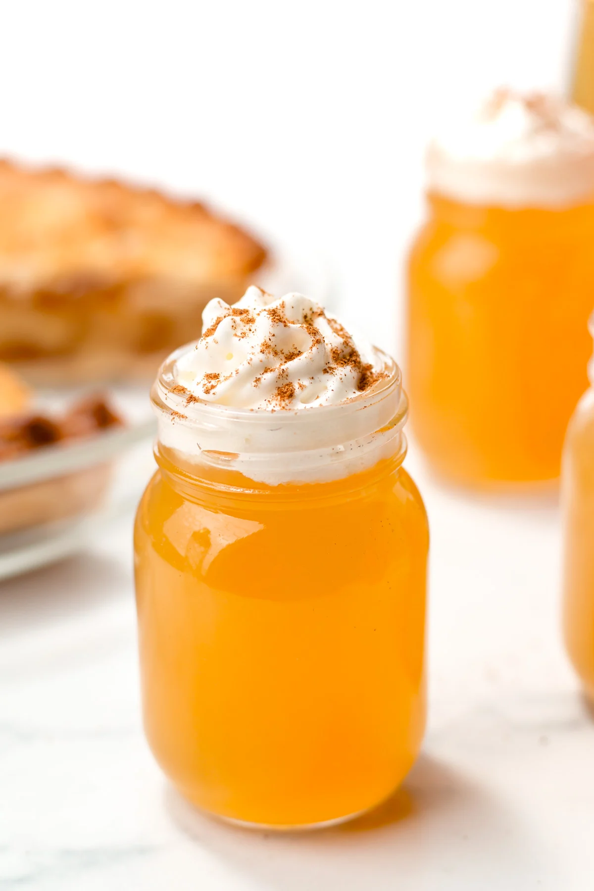
- 1 gallon apple cider
- 1 gallon apple juice
- 1 ½ cups white sugar, or to taste
- 6 (3 inch) cinnamon sticks
- 1 (1 liter) bottle 190 proof grain alcohol (such as Everclear)
Directions
- Inspect 9 (quart-sized) jars for cracks and rings for rust, discarding any defective ones. Immerse in simmering water until drink mix is ready. Wash new, unused lids and rings in warm soapy water.
- Combine apple cider, apple juice, sugar, and cinnamon sticks in a large pot over medium-high heat; bring to a boil, stirring until sugar has dissolved. Off heat, discard cinnamon sticks. Cool mixture to room temperature, about 4 hours; stir in grain alcohol.
- Pour drink mix into sterilized canning jars. Wipe rims with a moist paper towel to remove any residue. Top with lids and screw rings on tightly. Store in the refrigerator for up to 6 months.
:max_bytes(150000):strip_icc():format(webp)/AR-260471-loaded-breakfast-skillet-ddmfs-4x3-step-01-f192b72ea6224a11b99fbaf4a93cd476.jpg) Dotdash Meredith Food Studios
Dotdash Meredith Food Studios:max_bytes(150000):strip_icc():format(webp)/AR-260471-loaded-breakfast-skillet-ddmfs-4x3-step-02-ea00bb2cfc99430398176842d2dee6f5.jpg) Dotdash Meredith Food Studios
Dotdash Meredith Food Studios:max_bytes(150000):strip_icc():format(webp)/AR-260471-loaded-breakfast-skillet-ddmfs-4x3-step-03-ca9522e6fe644579a9d3d98b8a98dcc4.jpg) Dotdash Meredith Food Studios
Dotdash Meredith Food Studios:max_bytes(150000):strip_icc():format(webp)/AR-260471-loaded-breakfast-skillet-ddmfs-4x3-step-04-a8f023103d8649f1ae836cc150d1391b.jpg) Dotdash Meredith Food Studios
Dotdash Meredith Food Studios:max_bytes(150000):strip_icc():format(webp)/AR-260471-loaded-breakfast-skillet-ddmfs-4x3-step-05-fe673251472344a68a816e77f76b822a.jpg) Dotdash Meredith Food Studios
Dotdash Meredith Food Studios:max_bytes(150000):strip_icc():format(webp)/AR-260471-loaded-breakfast-skillet-ddmfs-4x3-step-06-e2c449816517445b9e613e769bc07bf9.jpg) Dotdash Meredith Food Studios
Dotdash Meredith Food Studios:max_bytes(150000):strip_icc():format(webp)/AR-260471-loaded-breakfast-skillet-ddmfs-4x3-step-07-97874aaabd174b4b9c0e531cbf62799d.jpg) Dotdash Meredith Food Studios
Dotdash Meredith Food Studios
:max_bytes(150000):strip_icc():format(webp)/AR-278443--Easy-Breakfast-Egg-Muffins-gw-ddmfs-4x3-step-01-c2d654dfd7284e7491891d03bf5b685d.jpg) Grant Webster / Food Stylist: Holly Dreesman / Prop Stylist: Gabe Greco
Grant Webster / Food Stylist: Holly Dreesman / Prop Stylist: Gabe Greco:max_bytes(150000):strip_icc():format(webp)/AR-278443--Easy-Breakfast-Egg-Muffins-gw-ddmfs-4x3-step-03-d83d4b34e0f14607b51ca6a5fdf43f54.jpg) Grant Webster / Food Stylist: Holly Dreesman / Prop Stylist: Gabe Greco
Grant Webster / Food Stylist: Holly Dreesman / Prop Stylist: Gabe Greco:max_bytes(150000):strip_icc():format(webp)/AR-278443--Easy-Breakfast-Egg-Muffins-gw-ddmfs-4x3-step-04-dd8ff226abca4ce385d8e276ee9727b4.jpg) Grant Webster / Food Stylist: Holly Dreesman / Prop Stylist: Gabe Greco
Grant Webster / Food Stylist: Holly Dreesman / Prop Stylist: Gabe Greco:max_bytes(150000):strip_icc():format(webp)/AR-278443--Easy-Breakfast-Egg-Muffins-gw-ddmfs-4x3-step-05-96df619620fc4004af01a0f290b54d69.jpg) Grant Webster / Food Stylist: Holly Dreesman / Prop Stylist: Gabe Greco
Grant Webster / Food Stylist: Holly Dreesman / Prop Stylist: Gabe Greco:max_bytes(150000):strip_icc():format(webp)/AR-278443--Easy-Breakfast-Egg-Muffins-gw-ddmfs-4x3-step-06-1ad6f639b1c441fd8d52bcce80460606.jpg) Grant Webster / Food Stylist: Holly Dreesman / Prop Stylist: Gabe Greco
Grant Webster / Food Stylist: Holly Dreesman / Prop Stylist: Gabe Greco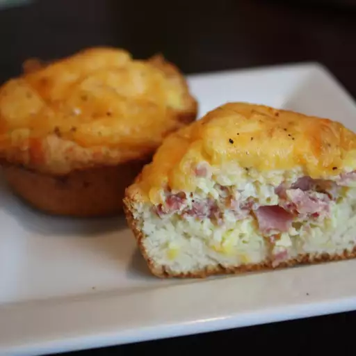
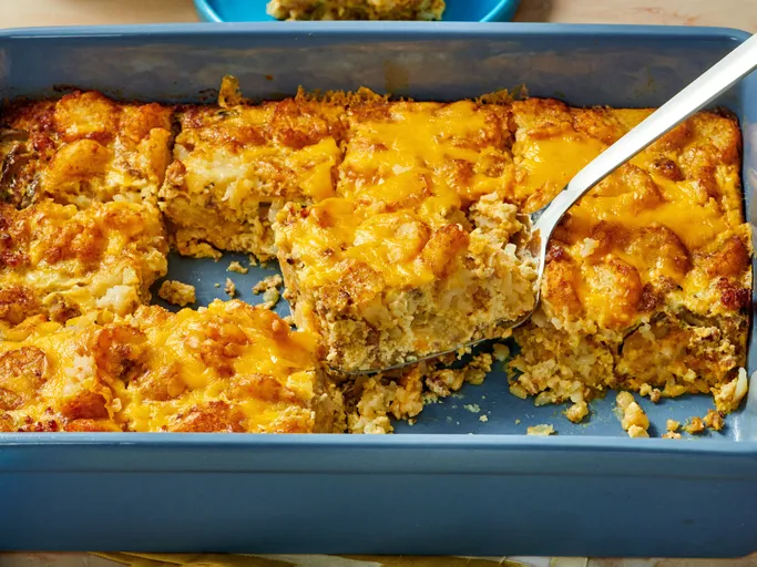
:max_bytes(150000):strip_icc():format(webp)/20701-breakfast-casserole-VAT-step-01-6195e80360d04bbcbeb31cfa04b4fd88.jpg) Allrecipes / Qi Ai
Allrecipes / Qi Ai:max_bytes(150000):strip_icc():format(webp)/20701-breakfast-casserole-VAT-step-02-93ac2a3f88504f369cbd712227c34431.jpg) Allrecipes / Qi Ai
Allrecipes / Qi Ai:max_bytes(150000):strip_icc():format(webp)/20701-breakfast-casserole-VAT-step-03-f191b40cc2564943a4e4fb69b56861d9.jpg) Allrecipes / Qi Ai
Allrecipes / Qi Ai:max_bytes(150000):strip_icc():format(webp)/20701-breakfast-casserole-VAT-step-04-541e63d66ab84f54a8b45e10f4765c0d.jpg) Allrecipes / Qi Ai
Allrecipes / Qi Ai