In this chapter, we will focus on the basic example of linear regression implementation using TensorFlow. Logistic regression or linear regression is a supervised machine learning approach for the classification of order discrete categories. Our goal in this chapter is to build a model by which a user can predict the relationship between predictor variables and one or more independent variables.
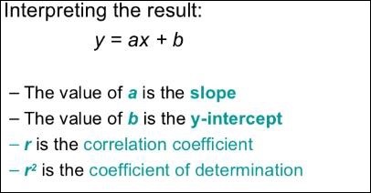
The relationship between these two variables is cons −idered linear. If y is the dependent variable and x is considered as the independent variable, then the linear regression relationship of two variables will look like the following equation −
Y = Ax+b
We will design an algorithm for linear regression. This will allow us to understand the following two important concepts −
Cost Function
Gradient descent algorithms
The schematic representation of linear regression is mentioned below −
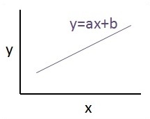
The graphical view of the equation of linear regression is mentioned below −
Steps to design an algorithm for linear regression
We will now learn about the steps that help in designing an algorithm for linear regression.
Step 1
It is important to import the necessary modules for plotting the linear regression module. We start importing the Python library NumPy and Matplotlib.
import numpy as np
import matplotlib.pyplot as plt
Step 2
Define the number of coefficients necessary for logistic regression.
number_of_points = 500
x_point = []
y_point = []
a = 0.22
b = 0.78
Step 3
Iterate the variables for generating 300 random points around the regression equation −
Y = 0.22x+0.78
for i in range(number_of_points):
   x = np.random.normal(0.0,0.5)
   y = a*x + b +np.random.normal(0.0,0.1) x_point.append([x])
   y_point.append([y])
The complete code for logistic regression is as follows −
import numpy as np
import matplotlib.pyplot as plt
number_of_points = 500
x_point = []
y_point = []
a = 0.22
b = 0.78
for i in range(number_of_points):
x = np.random.normal(0.0,0.5)
y = a*x + b +np.random.normal(0.0,0.1) x_point.append([x])
y_point.append([y])
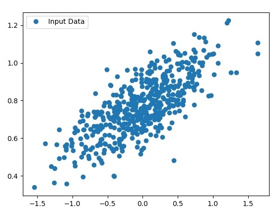
plt.plot(x_point,y_point, 'o', label = 'Input Data') plt.legend()
plt.show()
The number of points which is taken as input is considered as input data.
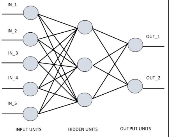
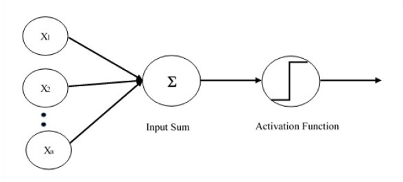
For understanding single layer perceptron, it is important to understand Artificial Neural Networks (ANN). Artificial neural networks is the information processing system the mechanism of which is inspired with the functionality of biological neural circuits. An artificial neural network possesses many processing units connected to each other. Following is the schematic representation of artificial neural network −
The diagram shows that the hidden units communicate with the external layer. While the input and output units communicate only through the hidden layer of the network.
The pattern of connection with nodes, the total number of layers and level of nodes between inputs and outputs with the number of neurons per layer define the architecture of a neural network.
There are two types of architecture. These types focus on the functionality artificial neural networks as follows −
Single Layer Perceptron
Multi-Layer Perceptron
Single Layer Perceptron
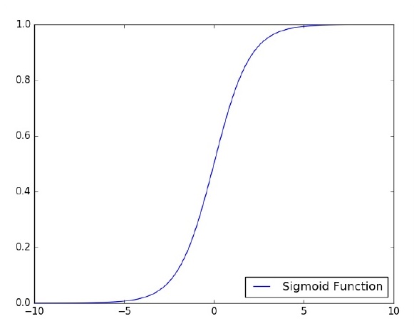
Single layer perceptron is the first proposed neural model created. The content of the local memory of the neuron consists of a vector of weights. The computation of a single layer perceptron is performed over the calculation of sum of the input vector each with the value multiplied by corresponding element of vector of the weights. The value which is displayed in the output will be the input of an activation function.
Let us focus on the implementation of single layer perceptron for an image classification problem using TensorFlow. The best example to illustrate the single layer perceptron is through representation of “Logistic Regression”.
Now, let us consider the following basic steps of training logistic regression −
The weights are initialized with random values at the beginning of the training.
For each element of the training set, the error is calculated with the difference between desired output and the actual output. The error calculated is used to adjust the weights.
The process is repeated until the error made on the entire training set is not less than the specified threshold, until the maximum number of iterations is reached.
The complete code for evaluation of logistic regression is mentioned below −
# Import MINST data
from tensorflow.examples.tutorials.mnist import input_data
mnist = input_data.read_data_sets("/tmp/data/", one_hot = True)
import tensorflow as tf
import matplotlib.pyplot as plt
# Parameters
learning_rate = 0.01
training_epochs = 25
batch_size = 100
display_step = 1
# tf Graph Input
x = tf.placeholder("float", [None, 784]) # mnist data image of shape 28*28 = 784
y = tf.placeholder("float", [None, 10]) # 0-9 digits recognition => 10 classes
# Create model
# Set model weights
W = tf.Variable(tf.zeros([784, 10]))
b = tf.Variable(tf.zeros([10]))
# Construct model
activation = tf.nn.softmax(tf.matmul(x, W) + b) # Softmax
# Minimize error using cross entropy
cross_entropy = y*tf.log(activation)
cost = tf.reduce_mean\ (-tf.reduce_sum\ (cross_entropy,reduction_indices = 1))
optimizer = tf.train.\ GradientDescentOptimizer(learning_rate).minimize(cost)
#Plot settings
avg_set = []
epoch_set = []
# Initializing the variables init = tf.initialize_all_variables()
# Launch the graph
with tf.Session() as sess:
sess.run(init)
# Training cycle
for epoch in range(training_epochs):
avg_cost = 0.
total_batch = int(mnist.train.num_examples/batch_size)
# Loop over all batches
for i in range(total_batch):
batch_xs, batch_ys = \ mnist.train.next_batch(batch_size)
# Fit training using batch data sess.run(optimizer, \ feed_dict = {
x: batch_xs, y: batch_ys})
# Compute average loss avg_cost += sess.run(cost, \ feed_dict = {
x: batch_xs, \ y: batch_ys})/total_batch
# Display logs per epoch step
if epoch % display_step == 0:
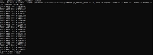
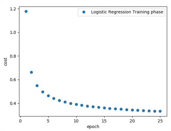
print ("Epoch:", '%04d' % (epoch+1), "cost=", "{:.9f}".format(avg_cost))
avg_set.append(avg_cost) epoch_set.append(epoch+1)
The logistic regression is considered as a predictive analysis. Logistic regression is used to describe data and to explain the relationship between one dependent binary variable and one or more nominal or independent variables.
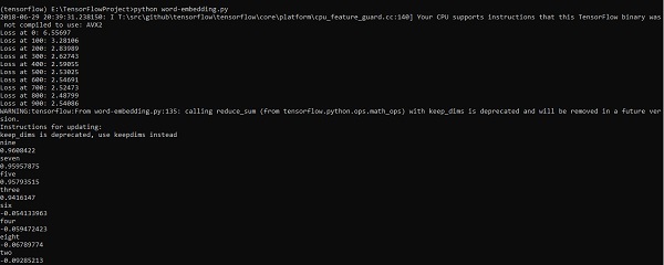
Word embedding is the concept of mapping from discrete objects such as words to vectors and real numbers. It is important for input for machine learning. The concept includes standard functions, which effectively transform discrete input objects to useful vectors.
The sample illustration of input of word embedding is as shown below −
Word2vec is the most common approach used for unsupervised word embedding technique. It trains the model in such a way that a given input word predicts the word’s context by using skip-grams.
TensorFlow enables many ways to implement this kind of model with increasing levels of sophistication and optimization and using multithreading concepts and higher-level abstractions.
import os
import math
import numpy as np
import tensorflow as tf
from tensorflow.contrib.tensorboard.plugins import projector
batch_size = 64
embedding_dimension = 5
negative_samples = 8
LOG_DIR = "logs/word2vec_intro"
digit_to_word_map = {
1: "One",
2: "Two",
3: "Three",
4: "Four",
5: "Five",
6: "Six",
7: "Seven",
8: "Eight",
9: "Nine"}
sentences = []
# Create two kinds of sentences - sequences of odd and even digits.
for i in range(10000):
rand_odd_ints = np.random.choice(range(1, 10, 2), 3)
sentences.append(" ".join([digit_to_word_map[r] for r in rand_odd_ints]))
sentences.append(" ".join([digit_to_word_map[r] for r in rand_even_ints]))
# Map words to indices
word2index_map = {}
index = 0
for sent in sentences:
for word in sent.lower().split():
if word not in word2index_map:
word2index_map[word] = index
index += 1
index2word_map = {index: word for word, index in word2index_map.items()}
vocabulary_size = len(index2word_map)
# Generate skip-gram pairs
skip_gram_pairs = []
for sent in sentences:
tokenized_sent = sent.lower().split()
for i in range(1, len(tokenized_sent)-1):
batch = instance_indices[:batch_size]
x = [skip_gram_pairs[i][0] for i in batch]
y = [[skip_gram_pairs[i][1]] for i in batch]
return x, y
# batch example
x_batch, y_batch = get_skipgram_batch(8)
x_batch
y_batch
[index2word_map[word] for word in x_batch] [index2word_map[word[0]] for word in y_batch]
# Input data, labels train_inputs = tf.placeholder(tf.int32, shape = [batch_size])
train_labels = tf.placeholder(tf.int32, shape = [batch_size, 1])
# Embedding lookup table currently only implemented in CPU with
tf.name_scope("embeddings"):
embeddings = tf.Variable(
tf.random_uniform([vocabulary_size, embedding_dimension], -1.0, 1.0),
name = 'embedding')
# This is essentialy a lookup table
embed = tf.nn.embedding_lookup(embeddings, train_inputs)
# Create variables for the NCE loss
nce_weights = tf.Variable(
tf.truncated_normal([vocabulary_size, embedding_dimension], stddev = 1.0 /
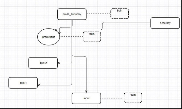
TensorFlow includes a visualization tool, which is called the TensorBoard. It is used for analyzing Data Flow Graph and also used to understand machine-learning models. The important feature of TensorBoard includes a view of different types of statistics about the parameters and details of any graph in vertical alignment.
Deep neural network includes up to 36,000 nodes. TensorBoard helps in collapsing these nodes in high-level blocks and highlighting the identical structures. This allows better analysis of graph focusing on the primary sections of the computation graph. The TensorBoard visualization is said to be very interactive where a user can pan, zoom and expand the nodes to display the details.
The following schematic diagram representation shows the complete working of TensorBoard visualization −
The algorithms collapse nodes into high-level blocks and highlight the specific groups with identical structures, which separate high-degree nodes. The TensorBoard thus created is useful and is treated equally important for tuning a machine learning model. This visualization tool is designed for the configuration log file with summary information and details that need to be displayed.
Let us focus on the demo example of TensorBoard visualization with the help of the following code −
import tensorflow as tf

# Constants creation for TensorBoard visualization
a = tf.constant(10,name = "a")
b = tf.constant(90,name = "b")
y = tf.Variable(a+b*2,name = 'y')
model = tf.initialize_all_variables() #Creation of model

with tf.Session() as session:
   merged = tf.merge_all_summaries()
   writer = tf.train.SummaryWriter("/tmp/tensorflowlogs",session.graph)
   session.run(model)
   print(session.run(y))
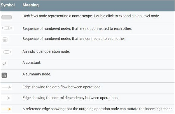
The following table shows the various symbols of TensorBoard visualization used for the node representation −
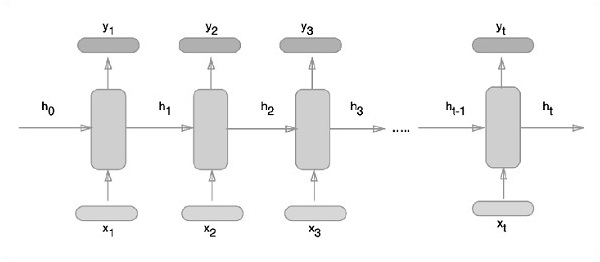
Recurrent neural networks is a type of deep learning-oriented algorithm, which follows a sequential approach. In neural networks, we always assume that each input and output is independent of all other layers. These type of neural networks are called recurrent because they perform mathematical computations in sequential manner.
Consider the following steps to train a recurrent neural network −
Step 1 − Input a specific example from dataset.
Step 2 − Network will take an example and compute some calculations using randomly initialized variables.
Step 3 − A predicted result is then computed.
Step 4 − The comparison of actual result generated with the expected value will produce an error.
Step 5 − To trace the error, it is propagated through same path where the variables are also adjusted.
Step 6 − The steps from 1 to 5 are repeated until we are confident that the variables declared to get the output are defined properly.
Step 7 − A systematic prediction is made by applying these variables to get new unseen input.
The schematic approach of representing recurrent neural networks is described below −
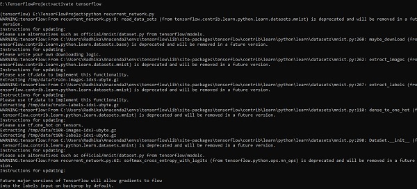
Recurrent Neural Network Implementation with TensorFlow
In this section, we will learn how to implement recurrent neural network with TensorFlow.
Step 1 − TensorFlow includes various libraries for specific implementation of the recurrent neural network module.
#Import necessary modules
from __future__ import print_function

import tensorflow as tf
from tensorflow.contrib import rnn
from tensorflow.examples.tutorials.mnist import input_data
mnist = input_data.read_data_sets("/tmp/data/", one_hot = True)
As mentioned above, the libraries help in defining the input data, which forms the primary part of recurrent neural network implementation.
Step 2 − Our primary motive is to classify the images using a recurrent neural network, where we consider every image row as a sequence of pixels. MNIST image shape is specifically defined as 28*28 px. Now we will handle 28 sequences of 28 steps for each sample that is mentioned. We will define the input parameters to get the sequential pattern done.
Step 3 − Compute the results using a defined function in RNN to get the best results. Here, each data shape is compared with current input shape and the results are computed to maintain the accuracy rate.
def RNN(x, weights, biases):
   x = tf.unstack(x, n_steps, 1)

   # Define a lstm cell with tensorflow
   lstm_cell = rnn.BasicLSTMCell(n_hidden, forget_bias=1.0)

   # Get lstm cell output
   outputs, states = rnn.static_rnn(lstm_cell, x, dtype = tf.float32)

   # Linear activation, using rnn inner loop last output
   return tf.matmul(outputs[-1], weights['out']) + biases['out']

pred = RNN(x, weights, biases)

# Define loss and optimizer
cost = tf.reduce_mean(tf.nn.softmax_cross_entropy_with_logits(logits = pred, labels = y))
optimizer = tf.train.AdamOptimizer(learning_rate = learning_rate).minimize(cost)

# Evaluate model
correct_pred = tf.equal(tf.argmax(pred,1), tf.argmax(y,1))
accuracy = tf.reduce_mean(tf.cast(correct_pred, tf.float32))

# Initializing the variables
init = tf.global_variables_initializer()
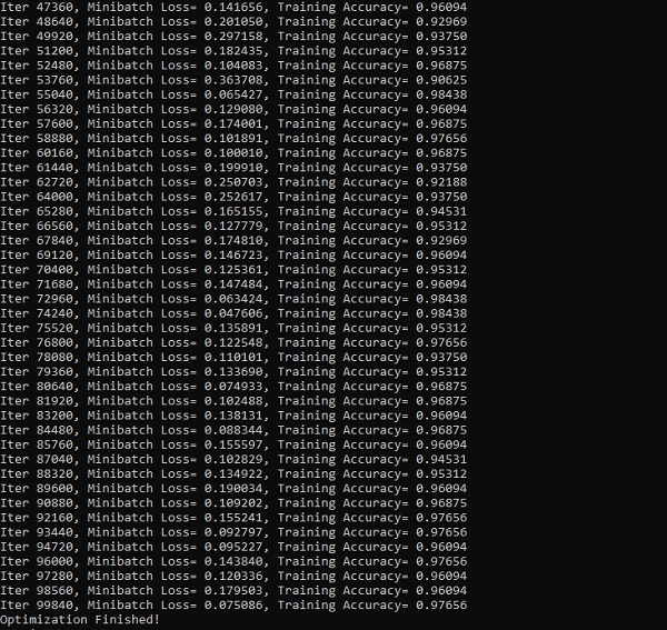
Step 4 − In this step, we will launch the graph to get the computational results. This also helps in calculating the accuracy for test results.
with tf.Session() as sess:
sess.run(init)
step = 1
# Keep training until reach max iterations
while step * batch_size < training_iters:
After understanding machine-learning concepts, we can now shift our focus to deep learning concepts. Deep learning is a division of machine learning and is considered as a crucial step taken by researchers in recent decades. The examples of deep learning implementation include applications like image recognition and speech recognition.
Following are the two important types of deep neural networks −
Convolutional Neural Networks
Recurrent Neural Networks
In this chapter, we will focus on the CNN, Convolutional Neural Networks.
Convolutional Neural Networks
Convolutional Neural networks are designed to process data through multiple layers of arrays. This type of neural networks is used in applications like image recognition or face recognition. The primary difference between CNN and any other ordinary neural network is that CNN takes input as a two-dimensional array and operates directly on the images rather than focusing on feature extraction which other neural networks focus on.
The dominant approach of CNN includes solutions for problems of recognition. Top companies like Google and Facebook have invested in research and development towards recognition projects to get activities done with greater speed.
A convolutional neural network uses three basic ideas −
Local respective fields
Convolution
Pooling
Let us understand these ideas in detail.
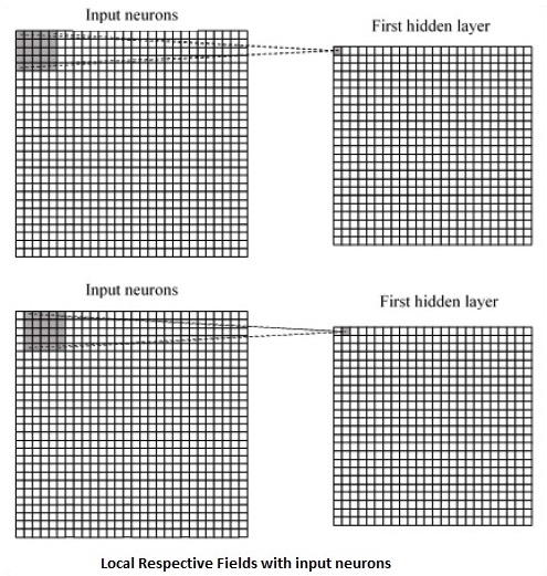
CNN utilizes spatial correlations that exist within the input data. Each concurrent layer of a neural network connects some input neurons. This specific region is called local receptive field. Local receptive field focusses on the hidden neurons. The hidden neurons process the input data inside the mentioned field not realizing the changes outside the specific boundary.
Following is a diagram representation of generating local respective fields −
If we observe the above representation, each connection learns a weight of the hidden neuron with an associated connection with movement from one layer to another. Here, individual neurons perform a shift from time to time. This process is called “convolution”.
The mapping of connections from the input layer to the hidden feature map is defined as “shared weights” and bias included is called “shared bias”.
CNN or convolutional neural networks use pooling layers, which are the layers, positioned immediately after CNN declaration. It takes the input from the user as a feature map that comes out of convolutional networks and prepares a condensed feature map. Pooling layers helps in creating layers with neurons of previous layers.
TensorFlow Implementation of CNN
In this section, we will learn about the TensorFlow implementation of CNN. The steps,which require the execution and proper dimension of the entire network, are as shown below −
Step 1 − Include the necessary modules for TensorFlow and the data set modules, which are needed to compute the CNN model.
import tensorflow as tf
import numpy as np
from tensorflow.examples.tutorials.mnist import input_data
Step 2 − Declare a function called run_cnn(), which includes various parameters and optimization variables with declaration of data placeholders. These optimization variables will declare the training pattern.
Step 3 − In this step, we will declare the training data placeholders with input parameters – for 28 x 28 pixels = 784. This is the flattened image data that is drawn from mnist.train.nextbatch().
We can reshape the tensor according to our requirements. The first value (-1) tells function to dynamically shape that dimension based on the amount of data passed to it. The two middle dimensions are set to the image size (i.e. 28 x 28).
x = tf.placeholder(tf.float32, [None, 784])
x_shaped = tf.reshape(x, [-1, 28, 28, 1])
y = tf.placeholder(tf.float32, [None, 10])
Step 4 − Now it is important to create some convolutional layers −
Step 5 − Let us flatten the output ready for the fully connected output stage – after two layers of stride 2 pooling with the dimensions of 28 x 28, to dimension of 14 x 14 or minimum 7 x 7 x,y co-ordinates, but with 64 output channels. To create the fully connected with “dense” layer, the new shape needs to be [-1, 7 x 7 x 64]. We can set up some weights and bias values for this layer, then activate with ReLU.
Step 6 − Another layer with specific softmax activations with the required optimizer defines the accuracy assessment, which makes the setup of initialization operator.
return out_layer
if __name__ == "__main__":
run_cnn()
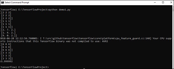
Following is the output generated by the above code −
See @{tf.nn.softmax_cross_entropy_with_logits_v2}.

2018-09-19 17:22:58.802268: I
T:\src\github\tensorflow\tensorflow\core\platform\cpu_feature_guard.cc:140]
Your CPU supports instructions that this TensorFlow binary was not compiled to
use: AVX2

2018-09-19 17:25:41.522845: W
T:\src\github\tensorflow\tensorflow\core\framework\allocator.cc:101] Allocation
of 1003520000 exceeds 10% of system memory.

2018-09-19 17:25:44.630941: W
T:\src\github\tensorflow\tensorflow\core\framework\allocator.cc:101] Allocation
of 501760000 exceeds 10% of system memory.

Epoch: 1 cost = 0.676 test accuracy: 0.940

2018-09-19 17:26:51.987554: W
T:\src\github\tensorflow\tensorflow\core\framework\allocator.cc:101] Allocation
of 1003520000 exceeds 10% of system memory.
In this chapter, we will learn about the basics of TensorFlow. We will begin by understanding the data structure of tensor.
Tensor Data Structure
Tensors are used as the basic data structures in TensorFlow language. Tensors represent the connecting edges in any flow diagram called the Data Flow Graph. Tensors are defined as multidimensional array or list.
Tensors are identified by the following three parameters −
Rank
Unit of dimensionality described within tensor is called rank. It identifies the number of dimensions of the tensor. A rank of a tensor can be described as the order or n-dimensions of a tensor defined.
Shape
The number of rows and columns together define the shape of Tensor.
Type
Type describes the data type assigned to Tensor’s elements.
A user needs to consider the following activities for building a Tensor −
Build an n-dimensional array
Convert the n-dimensional array.
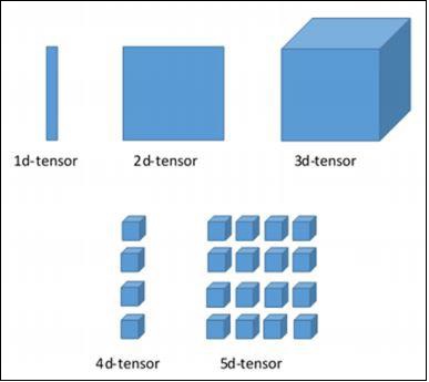
Various Dimensions of TensorFlow
TensorFlow includes various dimensions. The dimensions are described in brief below −
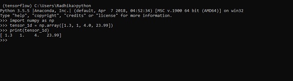
One dimensional Tensor
One dimensional tensor is a normal array structure which includes one set of values of the same data type.
The implementation with the output is shown in the screenshot below −
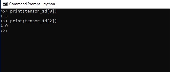
The indexing of elements is same as Python lists. The first element starts with index of 0; to print the values through index, all you need to do is mention the index number.
The above code will generate the following output −
Explanation
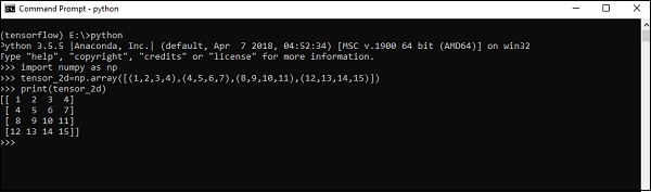
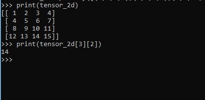
We have created multidimensional arrays in the above source code. Now, it is important to understand that we created graph and sessions, which manage the Tensors and generate the appropriate output. With the help of graph, we have the output specifying the mathematical calculations between Tensors.
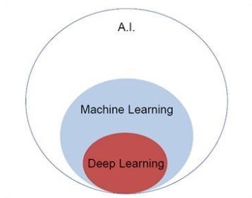
Artificial Intelligence is one of the most popular trends of recent times. Machine learning and deep learning constitute artificial intelligence. The Venn diagram shown below explains the relationship of machine learning and deep learning −
Machine Learning
Machine learning is the art of science of getting computers to act as per the algorithms designed and programmed. Many researchers think machine learning is the best way to make progress towards human-level AI. Machine learning includes the following types of patterns
Supervised learning pattern
Unsupervised learning pattern
Deep Learning
Deep learning is a subfield of machine learning where concerned algorithms are inspired by the structure and function of the brain called artificial neural networks.
All the value today of deep learning is through supervised learning or learning from labelled data and algorithms.
Each algorithm in deep learning goes through the same process. It includes a hierarchy of nonlinear transformation of input that can be used to generate a statistical model as output.
Consider the following steps that define the Machine Learning process
Identifies relevant data sets and prepares them for analysis.
Chooses the type of algorithm to use
Builds an analytical model based on the algorithm used.
Trains the model on test data sets, revising it as needed.
Runs the model to generate test scores.
Explore our latest online courses and learn new skills at your own pace. Enroll and become a certified expert to boost your career.
Difference between Machine Learning and Deep learning
In this section, we will learn about the difference between Machine Learning and Deep Learning.
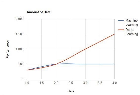
Amount of data
Machine learning works with large amounts of data. It is useful for small amounts of data too. Deep learning on the other hand works efficiently if the amount of data increases rapidly. The following diagram shows the working of machine learning and deep learning with the amount of data −
Hardware Dependencies
Deep learning algorithms are designed to heavily depend on high-end machines unlike the traditional machine learning algorithms. Deep learning algorithms perform a number of matrix multiplication operations, which require a large amount of hardware support.
Feature Engineering
Feature engineering is the process of putting domain knowledge into specified features to reduce the complexity of data and make patterns that are visible to learning algorithms it works.
Example − Traditional machine learning patterns focus on pixels and other attributes needed for feature engineering process. Deep learning algorithms focus on high-level features from data. It reduces the task of developing new feature extractor of every new problem.
Problem Solving Approach
The traditional machine learning algorithms follow a standard procedure to solve the problem. It breaks the problem into parts, solve each one of them and combine them to get the required result. Deep learning focusses in solving the problem from end to end instead of breaking them into divisions.
Execution Time
Execution time is the amount of time required to train an algorithm. Deep learning requires a lot of time to train as it includes a lot of parameters which takes a longer time than usual. Machine learning algorithm comparatively requires less execution time.
Interpretability
Interpretability is the major factor for comparison of machine learning and deep learning algorithms. The main reason is that deep learning is still given a second thought before its usage in industry.
Applications of Machine Learning and Deep Learning
In this section, we will learn about the different applications of Machine Learning and Deep Learning.
Computer vision which is used for facial recognition and attendance mark through fingerprints or vehicle identification through number plate.
Information Retrieval from search engines like text search for image search.
Automated email marketing with specified target identification.
Medical diagnosis of cancer tumors or anomaly identification of any chronic disease.
Natural language processing for applications like photo tagging. The best example to explain this scenario is used in Facebook.
Online Advertising.
Future Trends
With the increasing trend of using data science and machine learning in the industry, it will become important for each organization to inculcate machine learning in their businesses.
Deep learning is gaining more importance than machine learning. Deep learning is proving to be one of the best techniques in state-of-art performance.
Machine learning and deep learning will prove beneficial in research and academics field.
Conclusion
In this article, we had an overview of machine learning and deep learning with illustrations and differences also focusing on future trends. Many of AI applications utilize machine learning algorithms primarily to drive self-service, increase agent productivity and workflows more reliable. Machine learning and deep learning algorithms include an exciting prospect for many businesses and industry leaders.
It is important to understand mathematical concepts needed for TensorFlow before creating the basic application in TensorFlow. Mathematics is considered as the heart of any machine learning algorithm. It is with the help of core concepts of Mathematics, a solution for specific machine learning algorithm is defined.
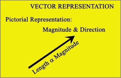
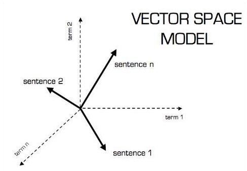
Vector
An array of numbers, which is either continuous or discrete, is defined as a vector. Machine learning algorithms deal with fixed length vectors for better output generation.
Machine learning algorithms deal with multidimensional data so vectors play a crucial role.
The pictorial representation of vector model is as shown below −
Scalar
Scalar can be defined as one-dimensional vector. Scalars are those, which include only magnitude and no direction. With scalars, we are only concerned with the magnitude.
Examples of scalar include weight and height parameters of children.
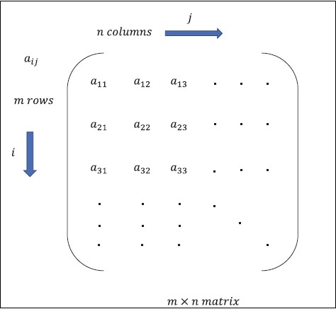
Matrix
Matrix can be defined as multi-dimensional arrays, which are arranged in the format of rows and columns. The size of matrix is defined by row length and column length. Following figure shows the representation of any specified matrix.
Consider the matrix with “m” rows and “n” columns as mentioned above, the matrix representation will be specified as “m*n matrix” which defined the length of matrix as well.
Mathematical Computations
In this section, we will learn about the different Mathematical Computations in TensorFlow.
Addition of matrices
Addition of two or more matrices is possible if the matrices are of the same dimension. The addition implies addition of each element as per the given position.
Consider the following example to understand how addition of matrices works −
The subtraction of matrices operates in similar fashion like the addition of two matrices. The user can subtract two matrices provided the dimensions are equal.
An Angular application consists mainly of components and their HTML templates. Because the components and templates provided by Angular cannot be understood by the browser directly, Angular applications require a compilation process before they can run in a browser.
The Angular ahead-of-time (AOT) compiler converts your Angular HTML and TypeScript code into efficient JavaScript code during the build phase before the browser downloads and runs that code. Compiling your application during the build process provides a faster rendering in the browser.
This guide explains how to specify metadata and apply available compiler options to compile your applications efficiently using the AOT compiler.
Watch Alex Rickabaugh explain the Angular compiler at AngularConnect 2019.
Here are some reasons you might want to use AOT.
Reasons
Details
Faster rendering
With AOT, the browser downloads a pre-compiled version of the application. The browser loads executable code so it can render the application immediately, without waiting to compile the application first.
Fewer asynchronous requests
The compiler inlines external HTML templates and CSS style sheets within the application JavaScript, eliminating separate ajax requests for those source files.
Smaller Angular framework download size
There’s no need to download the Angular compiler if the application is already compiled. The compiler is roughly half of Angular itself, so omitting it dramatically reduces the application payload.
Detect template errors earlier
The AOT compiler detects and reports template binding errors during the build step before users can see them.
Better security
AOT compiles HTML templates and components into JavaScript files long before they are served to the client. With no templates to read and no risky client-side HTML or JavaScript evaluation, there are fewer opportunities for injection attacks.
Choosing a compiler
Angular offers two ways to compile your application:
Angular compile
Details
Just-in-Time (JIT)
Compiles your application in the browser at runtime. This was the default until Angular 8.
Ahead-of-Time (AOT)
Compiles your application and libraries at build time. This is the default starting in Angular 9.
When you run the ng build (build only) or ng serve (build and serve locally) CLI commands, the type of compilation (JIT or AOT) depends on the value of the aot property in your build configuration specified in angular.json. By default, aot is set to true for new CLI applications.
See the CLI command reference and Building and serving Angular apps for more information.
How AOT works
The Angular AOT compiler extracts metadata to interpret the parts of the application that Angular is supposed to manage. You can specify the metadata explicitly in decorators such as @Component() and @Input(), or implicitly in the constructor declarations of the decorated classes. The metadata tells Angular how to construct instances of your application classes and interact with them at runtime.
In the following example, the @Component() metadata object and the class constructor tell Angular how to create and display an instance of TypicalComponent.
The Angular compiler extracts the metadata once and generates a factory for TypicalComponent. When it needs to create a TypicalComponent instance, Angular calls the factory, which produces a new visual element, bound to a new instance of the component class with its injected dependency.
Compilation phases
There are three phases of AOT compilation.
Phase
Details
1
code analysis
In this phase, the TypeScript compiler and AOT collector create a representation of the source. The collector does not attempt to interpret the metadata it collects. It represents the metadata as best it can and records errors when it detects a metadata syntax violation.
2
code generation
In this phase, the compiler’s StaticReflector interprets the metadata collected in phase 1, performs additional validation of the metadata, and throws an error if it detects a metadata restriction violation.
3
template type checking
In this optional phase, the Angular template compiler uses the TypeScript compiler to validate the binding expressions in templates. You can enable this phase explicitly by setting the strictTemplates configuration option; see Angular compiler options.
Metadata restrictions
You write metadata in a subset of TypeScript that must conform to the following general constraints:
Limit expression syntax to the supported subset of JavaScript
Only reference exported symbols after code folding
Only call functions supported by the compiler
Input/Outputs and data-bound class members must be public or protected.
For additional guidelines and instructions on preparing an application for AOT compilation, see Angular: Writing AOT-friendly applications.
Errors in AOT compilation commonly occur because of metadata that does not conform to the compiler’s requirements (as described more fully below). For help in understanding and resolving these problems, see AOT Metadata Errors.
Configuring AOT compilation
You can provide options in the TypeScript configuration file that controls the compilation process. See Angular compiler options for a complete list of available options.
Phase 1: Code analysis
The TypeScript compiler does some of the analytic work of the first phase. It emits the .d.tstype definition files with type information that the AOT compiler needs to generate application code. At the same time, the AOT collector analyzes the metadata recorded in the Angular decorators and outputs metadata information in .metadata.json files, one per .d.ts file.
You can think of .metadata.json as a diagram of the overall structure of a decorator’s metadata, represented as an abstract syntax tree (AST).
Angular’s schema.ts describes the JSON format as a collection of TypeScript interfaces.
Expression syntax limitations
The AOT collector only understands a subset of JavaScript. Define metadata objects with the following limited syntax:
Syntax
Example
Literal object
{cherry: true, apple: true, mincemeat: false}
Literal array
['cherries', 'flour', 'sugar']
Spread in literal array
['apples', 'flour', ...]
Calls
bake(ingredients)
New
new Oven()
Property access
pie.slice
Array index
ingredients[0]
Identity reference
Component
A template string
pie is ${multiplier} times better than cake
Literal string
'pi'
Literal number
3.14153265
Literal boolean
true
Literal null
null
Supported prefix operator
!cake
Supported binary operator
a+b
Conditional operator
a ? b : c
Parentheses
(a+b)
If an expression uses unsupported syntax, the collector writes an error node to the .metadata.json file. The compiler later reports the error if it needs that piece of metadata to generate the application code.
If you want ngc to report syntax errors immediately rather than produce a .metadata.json file with errors, set the strictMetadataEmit option in the TypeScript configuration file.
Angular libraries have this option to ensure that all Angular .metadata.json files are clean and it is a best practice to do the same when building your own libraries.
No arrow functions
The AOT compiler does not support function expressions and arrow functions, also called lambda functions.
The AOT collector does not support the arrow function, () => new Server(), in a metadata expression. It generates an error node in place of the function. When the compiler later interprets this node, it reports an error that invites you to turn the arrow function into an exported function.
You can fix the error by converting to this:
content_copyexport function serverFactory() {
  return new Server();
}

@Component({
  …
  providers: [{provide: server, useFactory: serverFactory}]
})
In version 5 and later, the compiler automatically performs this rewriting while emitting the .js file.
Code folding
The compiler can only resolve references to exported symbols. The collector, however, can evaluate an expression during collection and record the result in the .metadata.json, rather than the original expression. This allows you to make limited use of non-exported symbols within expressions.
For example, the collector can evaluate the expression 1 + 2 + 3 + 4 and replace it with the result, 10. This process is called folding. An expression that can be reduced in this manner is foldable.
The collector can evaluate references to module-local const declarations and initialized var and let declarations, effectively removing them from the .metadata.json file.
The compiler could not refer to the template constant because it isn’t exported. The collector, however, can fold the template constant into the metadata definition by in-lining its contents. The effect is the same as if you had written:
There is no longer a reference to template and, therefore, nothing to trouble the compiler when it later interprets the collector’s output in .metadata.json.
You can take this example a step further by including the template constant in another expression:
The following table describes which expressions the collector can and cannot fold:
Syntax
Foldable
Literal object
yes
Literal array
yes
Spread in literal array
no
Calls
no
New
no
Property access
yes, if target is foldable
Array index
yes, if target and index are foldable
Identity reference
yes, if it is a reference to a local
A template with no substitutions
yes
A template with substitutions
yes, if the substitutions are foldable
Literal string
yes
Literal number
yes
Literal boolean
yes
Literal null
yes
Supported prefix operator
yes, if operand is foldable
Supported binary operator
yes, if both left and right are foldable
Conditional operator
yes, if condition is foldable
Parentheses
yes, if the expression is foldable
If an expression is not foldable, the collector writes it to .metadata.json as an AST for the compiler to resolve.
Phase 2: code generation
The collector makes no attempt to understand the metadata that it collects and outputs to .metadata.json. It represents the metadata as best it can and records errors when it detects a metadata syntax violation. It’s the compiler’s job to interpret the .metadata.json in the code generation phase.
The compiler understands all syntax forms that the collector supports, but it may reject syntactically correct metadata if the semantics violate compiler rules.
Public or protected symbols
The compiler can only reference exported symbols.
Decorated component class members must be public or protected. You cannot make an @Input() property private.
Data bound properties must also be public or protected
Supported classes and functions
The collector can represent a function call or object creation with new as long as the syntax is valid. The compiler, however, can later refuse to generate a call to a particular function or creation of a particular object.
The compiler can only create instances of certain classes, supports only core decorators, and only supports calls to macros (functions or static methods) that return expressions.
Compiler action
Details
New instances
The compiler only allows metadata that create instances of the class InjectionToken from @angular/core.
Supported decorators
The compiler only supports metadata for the Angular decorators in the @angular/core module.
Function calls
Factory functions must be exported, named functions. The AOT compiler does not support lambda expressions (“arrow functions”) for factory functions.
Functions and static method calls
The collector accepts any function or static method that contains a single return statement. The compiler, however, only supports macros in the form of functions or static methods that return an expression.
For example, consider the following function:
content_copyexport function wrapInArray<T>(value: T): T[] {
  return [value];
}
You can call the wrapInArray in a metadata definition because it returns the value of an expression that conforms to the compiler’s restrictive JavaScript subset.
You might use wrapInArray() like this:
content_copy@NgModule({
  declarations: wrapInArray(TypicalComponent)
})
export class TypicalModule {}
The compiler treats this usage as if you had written:
content_copy@NgModule({
  declarations: [TypicalComponent]
})
export class TypicalModule {}
The Angular RouterModule exports two macro static methods, forRoot and forChild, to help declare root and child routes. Review the source code for these methods to see how macros can simplify configuration of complex NgModules.
Metadata rewriting
The compiler treats object literals containing the fields useClass, useValue, useFactory, and data specially, converting the expression initializing one of these fields into an exported variable that replaces the expression. This process of rewriting these expressions removes all the restrictions on what can be in them because the compiler doesn’t need to know the expression’s value —it just needs to be able to generate a reference to the value.
Without rewriting, this would be invalid because lambdas are not supported and TypicalServer is not exported. To allow this, the compiler automatically rewrites this to something like:
This allows the compiler to generate a reference to θ0 in the factory without having to know what the value of θ0 contains.
The compiler does the rewriting during the emit of the .js file. It does not, however, rewrite the .d.ts file, so TypeScript doesn’t recognize it as being an export. And it does not interfere with the ES module’s exported API.
Phase 3: Template type checking
One of the Angular compiler’s most helpful features is the ability to type-check expressions within templates, and catch any errors before they cause crashes at runtime. In the template type-checking phase, the Angular template compiler uses the TypeScript compiler to validate the binding expressions in templates.
Enable this phase explicitly by adding the compiler option "fullTemplateTypeCheck" in the "angularCompilerOptions" of the project’s TypeScript configuration file (see Angular Compiler Options).
Template validation produces error messages when a type error is detected in a template binding expression, similar to how type errors are reported by the TypeScript compiler against code in a .ts file.
my.component.ts.MyComponent.html(1,1): : Property 'addresss' does not exist on type 'Person'. Did you mean 'address'?
The file name reported in the error message, my.component.ts.MyComponent.html, is a synthetic file generated by the template compiler that holds contents of the MyComponent class template. The compiler never writes this file to disk. The line and column numbers are relative to the template string in the @Component annotation of the class, MyComponent in this case. If a component uses templateUrl instead of template, the errors are reported in the HTML file referenced by the templateUrl instead of a synthetic file.
The error location is the beginning of the text node that contains the interpolation expression with the error. If the error is in an attribute binding such as [value]="person.address.street", the error location is the location of the attribute that contains the error.
The validation uses the TypeScript type checker and the options supplied to the TypeScript compiler to control how detailed the type validation is. For example, if the strictTypeChecks is specified, the error
my.component.ts.MyComponent.html(1,1): : Object is possibly 'undefined'
is reported as well as the above error message.
Type narrowing
The expression used in an ngIf directive is used to narrow type unions in the Angular template compiler, the same way the if expression does in TypeScript. For example, to avoid Object is possibly 'undefined' error in the template above, modify it to only emit the interpolation if the value of person is initialized as shown below:
Using *ngIf allows the TypeScript compiler to infer that the person used in the binding expression will never be undefined.
For more information about input type narrowing, see Improving template type checking for custom directives.
Non-null type assertion operator
Use the non-null type assertion operator to suppress the Object is possibly 'undefined' error when it is inconvenient to use *ngIf or when some constraint in the component ensures that the expression is always non-null when the binding expression is interpolated.
In the following example, the person and address properties are always set together, implying that address is always non-null if person is non-null. There is no convenient way to describe this constraint to TypeScript and the template compiler, but the error is suppressed in the example by using address!.street.