Author: saqibkhan

Ingredients

1/2x1x2x

Original recipe (1X) yields 1 servings

• 1 cup ice, or as needed
• 3 fluid ounces grapefruit-flavored soda (such as Fresca)
• 2 fluid ounces white grapefruit juice
• 2 fluid ounces gin
• ½ fluid ounce freshly squeezed lemon juice
• 1 splash club soda, or as needed
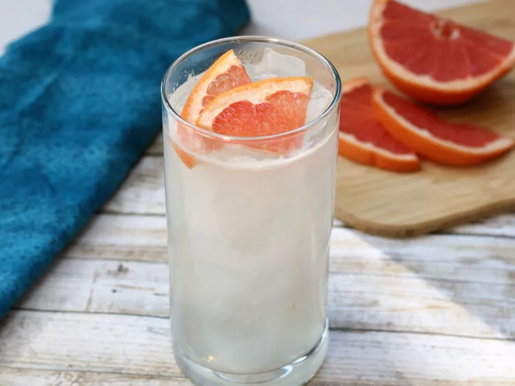
• 1 slice grapefruit for garnish

Directions

1. Fill a highball glass with ice. Add grapefruit soda, grapefruit juice, gin, and lemon juice; stir to combine. Top with club soda, lightly stir, and garnish with grapefruit slice.

Ingredients

Original recipe (1X) yields 8 servings

• 8 cups water, divided
• 1 cup quick-cooking oats
• 1 cinnamon stick
• ½ cup white sugar
• 2 teaspoons vanilla extract

Directions

1. Combine 5 cups water, quick-cooking oats, and cinnamon stick in a blender; blend until combined, about 1 minute.
2. Pour the oat mixture through a strainer, collecting the liquids in a pitcher and reserving the solids. Pour remaining water through the strainer containing the solids and into the pitcher. Add sugar and vanilla extract; refrigerate until chilled, about 1 hour.

Ingredients

Original recipe (1X) yields 1 servings

• ¼ cup frozen strawberries, thawed
• 1 ¼ fluid ounces amaretto liqueur
• 2 (1/2 cup) scoops vanilla ice cream
• 1 dash vanilla extract
• ½ cup crushed ice
• ¼ fluid ounce vanilla-flavored vodka
• 1 tablespoon whipped cream
• 1 fresh strawberry

Directions

1. Place thawed frozen strawberries, amaretto liqueur, vanilla ice cream, vanilla extract, crushed ice, and vanilla vodka into a blender.
2. Cover and blend until smooth.
3. Pour into a glass and garnish with whipped cream and a fresh strawberry.

Ingredients

Original recipe (1X) yields 1 servings

• 1 cup milk
• ½ cup cold brewed coffee
• 2 (1 gram) packets granular sucralose sweetener (such as Splenda®)

Directions

1. Mix milk, coffee, and sweetener together in a glass until sweetener is dissolved.

Ingredients

Original recipe (1X) yields 2 servings

• 2 bananas, sliced and frozen
• 1 cup unsweetened almond milk
• ½ cup canned pumpkin purée
• 1 scoop vanilla protein powder
• 2 dates, pitted
• ½ teaspoon vanilla extract
• 1 pinch ground nutmeg
• 1 pinch ground cinnamon
• 1 pinch ground cloves
• 1 pinch ground ginger

Directions

1. Combine bananas, almond milk, pumpkin purée, protein powder, dates, vanilla extract, nutmeg, cinnamon, cloves, and ginger in a blender; blend until smooth.

Ingredients

Original recipe (1X) yields 66 servings

• 1 cup white sugar
• 1 cup dry milk powder
• 1 cup powdered non-dairy creamer
• ½ cup unsweetened cocoa
• ¼ cup instant coffee granules

Directions

1. Combine sugar, milk powder, creamer, cocoa and instant coffee in a large bowl. Mix together until well blended. Store in a sealed container.
2. To serve: Heat a cup of water per serving (or milk, for a creamier taste). Stir in 2 to 3 heaping teaspoons of cocoa mixture.

Ingredients

Original recipe (1X) yields 1 servings

• ¾ cup almond milk
• 1 medium ripe banana
• 4 ice cubes
• 1 pinch ground cinnamon
• 1 dash vanilla extract

Directions

1. Combine almond milk, banana, ice cubes, cinnamon, and vanilla in a blender; blend on medium speed until frothy and smooth, about 1 minute.

Ingredients

Original recipe (1X) yields 4 servings

• 1 cup uncooked long grain white rice
• 3 ½ cups cold water
• 1 (12 fluid ounce) can evaporated milk
• ½ cup white sugar
• ½ teaspoon ground cinnamon
• 1 teaspoon vanilla extract

Directions

1. Place the rice in a bowl with enough water to cover it and let it soak overnight.
2. Strain the rice and discard the water. Stir the cold water and evaporated milk together. Place the drained rice into a blender along with half of the diluted milk. Blend until the rice is finely ground, about 30 seconds. Add the sugar, cinnamon, and vanilla; blend well. Pour in the remaining diluted milk; blend.
3. Line a strainer with two layers of cheesecloth. Place the strainer over another bowl to catch the liquid. Strain the rice milk through the cheesecloth, discard the solids. Repeat the process if necessary. Serve over ice.

Ingredients

Original recipe (1X) yields 6 servings

• ¾ cup chilled orange juice
• ⅓ cup chilled pineapple juice
• 2 cups vanilla yogurt
• 1 cup frozen blueberries
• ½ cup frozen sliced strawberries
• ½ banana, sliced

Directions

1. Place the orange juice, pineapple juice, yogurt, blueberries, strawberries, and bananas into a blender. Cover and blend until smooth. The berry drink will be very thick. Serve immediately.

Ingredients

Original recipe (1X) yields 1 servings

• 1 cup milk
• 1 teaspoon honey
• 2 drops vanilla extract
• 1 pinch ground cinnamon

Directions

1. Gather all ingredients.Dotdash Meredith Food Studios
2. Pour milk into a microwave-safe mug. Cook on high until milk is very hot and begins to foam, about 3 minutes.Dotdash Meredith Food Studios
3. Stir in honey and vanilla, then sprinkle with cinnamon before serving.