Author: saqibkhan

The binomial distribution model deals with finding the probability of success of an event which has only two possible outcomes in a series of experiments. For example, tossing of a coin always gives a head or a tail. The probability of finding exactly 3 heads in tossing a coin repeatedly for 10 times is estimated during the binomial distribution.

R has four in-built functions to generate binomial distribution. They are described below.

dbinom(x, size, prob)
pbinom(x, size, prob)
qbinom(p, size, prob)
rbinom(n, size, prob)

Following is the description of the parameters used −

• x is a vector of numbers.
• p is a vector of probabilities.
• n is number of observations.
• size is the number of trials.
• prob is the probability of success of each trial.

dbinom()

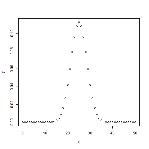
This function gives the probability density distribution at each point.

# Create a sample of 50 numbers which are incremented by 1.
x <- seq(0,50,by = 1)

# Create the binomial distribution.
y <- dbinom(x,50,0.5)

# Give the chart file a name.
png(file = "dbinom.png")

# Plot the graph for this sample.
plot(x,y)

# Save the file.
dev.off()

When we execute the above code, it produces the following result −

pbinom()

This function gives the cumulative probability of an event. It is a single value representing the probability.

# Probability of getting 26 or less heads from a 51 tosses of a coin.
x <- pbinom(26,51,0.5)

print(x)

When we execute the above code, it produces the following result −

[1] 0.610116

Explore our latest online courses and learn new skills at your own pace. Enroll and become a certified expert to boost your career.

qbinom()

This function takes the probability value and gives a number whose cumulative value matches the probability value.

# How many heads will have a probability of 0.25 will come out when a coin
# is tossed 51 times.
x <- qbinom(0.25,51,1/2)

print(x)

When we execute the above code, it produces the following result −

[1] 23

rbinom()

This function generates required number of random values of given probability from a given sample.

# Find 8 random values from a sample of 150 with probability of 0.4.
x <- rbinom(8,150,.4)

print(x)

When we execute the above code, it produces the following result −

[1] 58 61 59 66 55 60 61 67

In a random collection of data from independent sources, it is generally observed that the distribution of data is normal. Which means, on plotting a graph with the value of the variable in the horizontal axis and the count of the values in the vertical axis we get a bell shape curve. The center of the curve represents the mean of the data set. In the graph, fifty percent of values lie to the left of the mean and the other fifty percent lie to the right of the graph. This is referred as normal distribution in statistics.

R has four in built functions to generate normal distribution. They are described below.

dnorm(x, mean, sd)
pnorm(x, mean, sd)
qnorm(p, mean, sd)
rnorm(n, mean, sd)

Following is the description of the parameters used in above functions −

• x is a vector of numbers.
• p is a vector of probabilities.
• n is number of observations(sample size).
• mean is the mean value of the sample data. It’s default value is zero.
• sd is the standard deviation. It’s default value is 1.

dnorm()

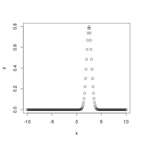
This function gives height of the probability distribution at each point for a given mean and standard deviation.

# Create a sequence of numbers between -10 and 10 incrementing by 0.1.
x <- seq(-10, 10, by = .1)

# Choose the mean as 2.5 and standard deviation as 0.5.
y <- dnorm(x, mean = 2.5, sd = 0.5)

# Give the chart file a name.
png(file = "dnorm.png")

plot(x,y)

# Save the file.
dev.off()

When we execute the above code, it produces the following result −

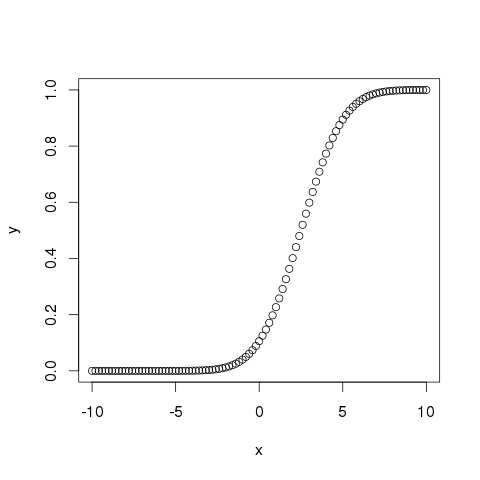
pnorm()

This function gives the probability of a normally distributed random number to be less that the value of a given number. It is also called “Cumulative Distribution Function”.

# Create a sequence of numbers between -10 and 10 incrementing by 0.2.
x <- seq(-10,10,by = .2)
 
# Choose the mean as 2.5 and standard deviation as 2. 
y <- pnorm(x, mean = 2.5, sd = 2)

# Give the chart file a name.
png(file = "pnorm.png")

# Plot the graph.
plot(x,y)

# Save the file.
dev.off()

When we execute the above code, it produces the following result −

Explore our latest online courses and learn new skills at your own pace. Enroll and become a certified expert to boost your career.

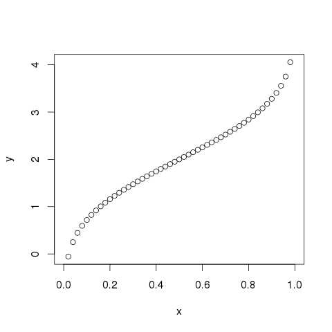
qnorm()

This function takes the probability value and gives a number whose cumulative value matches the probability value.

# Create a sequence of probability values incrementing by 0.02.
x <- seq(0, 1, by = 0.02)

# Choose the mean as 2 and standard deviation as 3.
y <- qnorm(x, mean = 2, sd = 1)

# Give the chart file a name.
png(file = "qnorm.png")

# Plot the graph.
plot(x,y)

# Save the file.
dev.off()

When we execute the above code, it produces the following result −

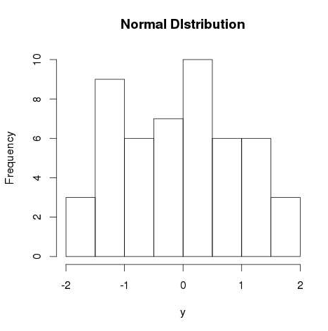
rnorm()

This function is used to generate random numbers whose distribution is normal. It takes the sample size as input and generates that many random numbers. We draw a histogram to show the distribution of the generated numbers.

# Create a sample of 50 numbers which are normally distributed.
y <- rnorm(50)

# Give the chart file a name.
png(file = "rnorm.png")

# Plot the histogram for this sample.
hist(y, main = "Normal DIstribution")

# Save the file.
dev.off()

When we execute the above code, it produces the following result −

The Logistic Regression is a regression model in which the response variable (dependent variable) has categorical values such as True/False or 0/1. It actually measures the probability of a binary response as the value of response variable based on the mathematical equation relating it with the predictor variables.

The general mathematical equation for logistic regression is −

y = 1/(1+e^-(a+b1x1+b2x2+b3x3+...))

Following is the description of the parameters used −

• y is the response variable.
• x is the predictor variable.
• a and b are the coefficients which are numeric constants.

The function used to create the regression model is the glm() function.

Syntax

The basic syntax for glm() function in logistic regression is −

glm(formula,data,family)

Following is the description of the parameters used −

• formula is the symbol presenting the relationship between the variables.
• data is the data set giving the values of these variables.
• family is R object to specify the details of the model. It’s value is binomial for logistic regression.

Example

The in-built data set “mtcars” describes different models of a car with their various engine specifications. In “mtcars” data set, the transmission mode (automatic or manual) is described by the column am which is a binary value (0 or 1). We can create a logistic regression model between the columns “am” and 3 other columns – hp, wt and cyl.

# Select some columns form mtcars.
input <- mtcars[,c("am","cyl","hp","wt")]

print(head(input))

When we execute the above code, it produces the following result −

                  am   cyl  hp    wt
Mazda RX4          1   6    110   2.620
Mazda RX4 Wag      1   6    110   2.875
Datsun 710         1   4     93   2.320
Hornet 4 Drive     0   6    110   3.215
Hornet Sportabout  0   8    175   3.440
Valiant            0   6    105   3.460

Create Regression Model

We use the glm() function to create the regression model and get its summary for analysis.

input <- mtcars[,c("am","cyl","hp","wt")]

am.data = glm(formula = am ~ cyl + hp + wt, data = input, family = binomial)

print(summary(am.data))

When we execute the above code, it produces the following result −

Call:
glm(formula = am ~ cyl + hp + wt, family = binomial, data = input)

Deviance Residuals: 
 Min        1Q      Median        3Q       Max  
-2.17272     -0.14907  -0.01464     0.14116   1.27641  

Coefficients:
        Estimate Std. Error z value Pr(>|z|)  
(Intercept) 19.70288    8.11637   2.428   0.0152 *
cyl          0.48760    1.07162   0.455   0.6491  
hp           0.03259    0.01886   1.728   0.0840 .
wt          -9.14947    4.15332  -2.203   0.0276 *
---
Signif. codes:  0 ‘***’ 0.001 ‘**’ 0.01 ‘*’ 0.05 ‘.’ 0.1 ‘ ’ 1

(Dispersion parameter for binomial family taken to be 1)

Null deviance: 43.2297  on 31  degrees of freedom
Residual deviance:  9.8415  on 28  degrees of freedom
AIC: 17.841

Number of Fisher Scoring iterations: 8

Conclusion

In the summary as the p-value in the last column is more than 0.05 for the variables “cyl” and “hp”, we consider them to be insignificant in contributing to the value of the variable “am”. Only weight (wt) impacts the “am” value in this regression model.

Multiple regression is an extension of linear regression into relationship between more than two variables. In simple linear relation we have one predictor and one response variable, but in multiple regression we have more than one predictor variable and one response variable.

The general mathematical equation for multiple regression is −

y = a + b1x1 + b2x2 +...bnxn

Following is the description of the parameters used −

• y is the response variable.
• a, b1, b2…bn are the coefficients.
• x1, x2, …xn are the predictor variables.

We create the regression model using the lm() function in R. The model determines the value of the coefficients using the input data. Next we can predict the value of the response variable for a given set of predictor variables using these coefficients.

lm() Function

This function creates the relationship model between the predictor and the response variable.

Syntax

The basic syntax for lm() function in multiple regression is −

lm(y ~ x1+x2+x3...,data)

Following is the description of the parameters used −

• formula is a symbol presenting the relation between the response variable and predictor variables.
• data is the vector on which the formula will be applied.

Example

Input Data

Consider the data set “mtcars” available in the R environment. It gives a comparison between different car models in terms of mileage per gallon (mpg), cylinder displacement(“disp”), horse power(“hp”), weight of the car(“wt”) and some more parameters.

The goal of the model is to establish the relationship between “mpg” as a response variable with “disp”,”hp” and “wt” as predictor variables. We create a subset of these variables from the mtcars data set for this purpose.

input <- mtcars[,c("mpg","disp","hp","wt")]
print(head(input))

When we execute the above code, it produces the following result −

                   mpg   disp   hp    wt
Mazda RX4          21.0  160    110   2.620
Mazda RX4 Wag      21.0  160    110   2.875
Datsun 710         22.8  108     93   2.320
Hornet 4 Drive     21.4  258    110   3.215
Hornet Sportabout  18.7  360    175   3.440
Valiant            18.1  225    105   3.460

Create Relationship Model & get the Coefficients

input <- mtcars[,c("mpg","disp","hp","wt")]

# Create the relationship model.
model <- lm(mpg~disp+hp+wt, data = input)

# Show the model.
print(model)

# Get the Intercept and coefficients as vector elements.
cat("# # # # The Coefficient Values # # # ","\n")

a <- coef(model)[1]
print(a)

Xdisp <- coef(model)[2]
Xhp <- coef(model)[3]
Xwt <- coef(model)[4]

print(Xdisp)
print(Xhp)
print(Xwt)

When we execute the above code, it produces the following result −

Call:
lm(formula = mpg ~ disp + hp + wt, data = input)

Coefficients:
(Intercept)         disp           hp           wt  
  37.105505      -0.000937        -0.031157    -3.800891  

# # # # The Coefficient Values # # # 
(Intercept) 
   37.10551 
     disp 
-0.0009370091 
     hp 
-0.03115655 
   wt 
-3.800891 

Create Equation for Regression Model

Based on the above intercept and coefficient values, we create the mathematical equation.

Y = a+Xdisp.x1+Xhp.x2+Xwt.x3
or
Y = 37.15+(-0.000937)*x1+(-0.0311)*x2+(-3.8008)*x3

Apply Equation for predicting New Values

We can use the regression equation created above to predict the mileage when a new set of values for displacement, horse power and weight is provided.

For a car with disp = 221, hp = 102 and wt = 2.91 the predicted mileage is −

Y = 37.15+(-0.000937)*221+(-0.0311)*102+(-3.8008)*2.91 = 22.7104

Regression analysis is a very widely used statistical tool to establish a relationship model between two variables. One of these variable is called predictor variable whose value is gathered through experiments. The other variable is called response variable whose value is derived from the predictor variable.

In Linear Regression these two variables are related through an equation, where exponent (power) of both these variables is 1. Mathematically a linear relationship represents a straight line when plotted as a graph. A non-linear relationship where the exponent of any variable is not equal to 1 creates a curve.

The general mathematical equation for a linear regression is −

y = ax + b

Following is the description of the parameters used −

• y is the response variable.
• x is the predictor variable.
• a and b are constants which are called the coefficients.

Steps to Establish a Regression

A simple example of regression is predicting weight of a person when his height is known. To do this we need to have the relationship between height and weight of a person.

The steps to create the relationship is −

• Carry out the experiment of gathering a sample of observed values of height and corresponding weight.
• Create a relationship model using the lm() functions in R.
• Find the coefficients from the model created and create the mathematical equation using these
• Get a summary of the relationship model to know the average error in prediction. Also called residuals.
• To predict the weight of new persons, use the predict() function in R.

Input Data

Below is the sample data representing the observations −

# Values of height
151, 174, 138, 186, 128, 136, 179, 163, 152, 131

# Values of weight.
63, 81, 56, 91, 47, 57, 76, 72, 62, 48

lm() Function

This function creates the relationship model between the predictor and the response variable.

Syntax

The basic syntax for lm() function in linear regression is −

lm(formula,data)

Following is the description of the parameters used −

• formula is a symbol presenting the relation between x and y.
• data is the vector on which the formula will be applied.

Create Relationship Model & get the Coefficients

x <- c(151, 174, 138, 186, 128, 136, 179, 163, 152, 131)
y <- c(63, 81, 56, 91, 47, 57, 76, 72, 62, 48)

# Apply the lm() function.
relation <- lm(y~x)

print(relation)

When we execute the above code, it produces the following result −

Call:
lm(formula = y ~ x)

Coefficients:
(Intercept)            x  
   -38.4551          0.6746 

Get the Summary of the Relationship

x <- c(151, 174, 138, 186, 128, 136, 179, 163, 152, 131)
y <- c(63, 81, 56, 91, 47, 57, 76, 72, 62, 48)

# Apply the lm() function.
relation <- lm(y~x)

print(summary(relation))

When we execute the above code, it produces the following result −

Call:
lm(formula = y ~ x)

Residuals:
Min      1Q     Median      3Q     Max 
-6.3002    -1.6629  0.0412    1.8944  3.9775 

Coefficients:
         Estimate Std. Error t value Pr(>|t|)    
(Intercept) -38.45509    8.04901  -4.778  0.00139 ** 
x             0.67461    0.05191  12.997 1.16e-06 ***
---
Signif. codes:  0 ‘***’ 0.001 ‘**’ 0.01 ‘*’ 0.05 ‘.’ 0.1 ‘ ’ 1

Residual standard error: 3.253 on 8 degrees of freedom
Multiple R-squared:  0.9548,    Adjusted R-squared:  0.9491 
F-statistic: 168.9 on 1 and 8 DF,  p-value: 1.164e-06

Explore our latest online courses and learn new skills at your own pace. Enroll and become a certified expert to boost your career.

predict() Function

Syntax

The basic syntax for predict() in linear regression is −

predict(object, newdata)

Following is the description of the parameters used −

• object is the formula which is already created using the lm() function.
• newdata is the vector containing the new value for predictor variable.

Predict the weight of new persons

# The predictor vector.
x <- c(151, 174, 138, 186, 128, 136, 179, 163, 152, 131)

# The resposne vector.
y <- c(63, 81, 56, 91, 47, 57, 76, 72, 62, 48)

# Apply the lm() function.
relation <- lm(y~x)

# Find weight of a person with height 170.
a <- data.frame(x = 170)
result <-  predict(relation,a)
print(result)

When we execute the above code, it produces the following result −

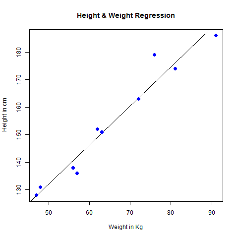
       1 
76.22869 

Visualize the Regression Graphically

# Create the predictor and response variable.
x <- c(151, 174, 138, 186, 128, 136, 179, 163, 152, 131)
y <- c(63, 81, 56, 91, 47, 57, 76, 72, 62, 48)
relation <- lm(y~x)

# Give the chart file a name.
png(file = "linearregression.png")

# Plot the chart.
plot(y,x,col = "blue",main = "Height & Weight Regression",
abline(lm(x~y)),cex = 1.3,pch = 16,xlab = "Weight in Kg",ylab = "Height in cm")

# Save the file.
dev.off()

When we execute the above code, it produces the following result −