- Package Development: R’s infrastructure supports easy package development, making it accessible for researchers and practitioners to share their work. The
devtoolspackage simplifies package creation, testing, and documentation. - Version Control and Collaboration: Tools like GitHub are widely used within the R community for version control and collaboration on projects. The integration with RStudio enhances this workflow.
- RStudio: An integrated development environment (IDE) that has become synonymous with R programming. It provides a user-friendly interface, built-in tools for package management, version control, and powerful debugging features.
Author: saqibkhan
-
Ecosystem and Package Management
-
Technical Features of R
- Data Structures: R’s foundational data structures include:
- Vectors: The basic building blocks for data in R, which can be numeric, character, or logical.
- Lists: Collections of objects that can be of different types, allowing for flexible data handling.
- Data Frames: A two-dimensional structure similar to tables in databases or spreadsheets, making it ideal for statistical analysis.
- Matrices: Two-dimensional arrays that can contain elements of the same type.
- Statistical Modeling: R excels in statistical modeling, offering a wide range of built-in functions and packages for linear models, generalized linear models, time series analysis, and more.
- Visualization: Beyond ggplot2, R has other visualization tools like lattice and base R plotting functions, allowing for various styles and customization options.
- Data Structures: R’s foundational data structures include:
-
Survival Analysis
Survival analysis deals with predicting the time when a specific event is going to occur. It is also known as failure time analysis or analysis of time to death. For example predicting the number of days a person with cancer will survive or predicting the time when a mechanical system is going to fail.
The R package named survival is used to carry out survival analysis. This package contains the function Surv() which takes the input data as a R formula and creates a survival object among the chosen variables for analysis. Then we use the function survfit() to create a plot for the analysis.
Install Package
install.packages("survival")Syntax
The basic syntax for creating survival analysis in R is −
Surv(time,event)
survfit(formula)
Following is the description of the parameters used −
- time is the follow up time until the event occurs.
- event indicates the status of occurrence of the expected event.
- formula is the relationship between the predictor variables.
Example
We will consider the data set named “pbc” present in the survival packages installed above. It describes the survival data points about people affected with primary biliary cirrhosis (PBC) of the liver. Among the many columns present in the data set we are primarily concerned with the fields “time” and “status”. Time represents the number of days between registration of the patient and earlier of the event between the patient receiving a liver transplant or death of the patient.
# Load the library.
library("survival")

# Print first few rows.
print(head(pbc))
When we execute the above code, it produces the following result and chart −
  id time status trt      age sex ascites hepato spiders edema bili chol
1  1  400      2   1 58.76523   f       1      1       1   1.0 14.5  261
2  2 4500      0   1 56.44627   f       0      1       1   0.0  1.1  302
3  3 1012      2   1 70.07255   m       0      0       0   0.5  1.4  176
4  4 1925      2   1 54.74059   f       0      1       1   0.5  1.8  244
5  5 1504      1   2 38.10541   f       0      1       1   0.0  3.4  279
6  6 2503      2   2 66.25873   f       0      1       0   0.0  0.8  248
  albumin copper alk.phos    ast trig platelet protime stage
1    2.60    156   1718.0 137.95  172      190    12.2     4
2    4.14     54   7394.8 113.52   88      221    10.6     3
3    3.48    210    516.0  96.10   55      151    12.0     4
4    2.54     64   6121.8  60.63   92      183    10.3     4
5    3.53    143    671.0 113.15   72      136    10.9     3
6    3.98     50    944.0  93.00   63       NA    11.0     3
From the above data we are considering time and status for our analysis.
Applying Surv() and survfit() Function
Now we proceed to apply the Surv() function to the above data set and create a plot that will show the trend.
# Load the library.
library("survival")

# Create the survival object.
survfit(Surv(pbc$time,pbc$status == 2)~1)

# Give the chart file a name.
png(file = "survival.png")

# Plot the graph.
plot(survfit(Surv(pbc$time,pbc$status == 2)~1))

# Save the file.
dev.off()
When we execute the above code, it produces the following result and chart −
Call: survfit(formula = Surv(pbc$time, pbc$status == 2) ~ 1)n events median 0.95LCL 0.95UCL 418 161 3395 3090 3853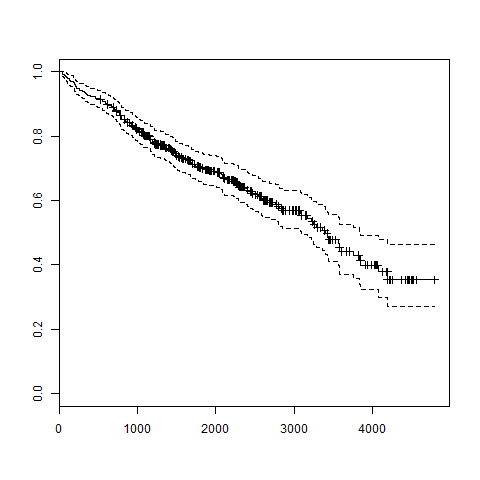
-
Random Forest
In the random forest approach, a large number of decision trees are created. Every observation is fed into every decision tree. The most common outcome for each observation is used as the final output. A new observation is fed into all the trees and taking a majority vote for each classification model.
An error estimate is made for the cases which were not used while building the tree. That is called an OOB (Out-of-bag) error estimate which is mentioned as a percentage.
The R package “randomForest” is used to create random forests.
Install R Package
Use the below command in R console to install the package. You also have to install the dependent packages if any.
install.packages("randomForest)The package “randomForest” has the function randomForest() which is used to create and analyze random forests.
Syntax
The basic syntax for creating a random forest in R is −
randomForest(formula, data)Following is the description of the parameters used −
- formula is a formula describing the predictor and response variables.
- data is the name of the data set used.
Input Data
We will use the R in-built data set named readingSkills to create a decision tree. It describes the score of someone’s readingSkills if we know the variables “age”,”shoesize”,”score” and whether the person is a native speaker.
Here is the sample data.
# Load the party package. It will automatically load other
# required packages.
library(party)

# Print some records from data set readingSkills.
print(head(readingSkills))
When we execute the above code, it produces the following result and chart −
  nativeSpeaker   age   shoeSize      score
1           yes     5   24.83189   32.29385
2           yes     6   25.95238   36.63105
3            no    11   30.42170   49.60593
4           yes     7   28.66450   40.28456
5           yes    11   31.88207   55.46085
6           yes    10   30.07843   52.83124
Loading required package: methods
Loading required package: grid
...............................
...............................
Example
We will use the randomForest() function to create the decision tree and see it’s graph.
# Load the party package. It will automatically load other # required packages. library(party) library(randomForest) # Create the forest. output.forest <- randomForest(nativeSpeaker ~ age + shoeSize + score,
# View the forest results. print(output.forest) # Importance of each predictor. print(importance(fit,type = 2))data = readingSkills)When we execute the above code, it produces the following result −
Call: randomForest(formula = nativeSpeaker ~ age + shoeSize + score,
No. of variables tried at each split: 1data = readingSkills) Type of random forest: classification Number of trees: 500
Confusion matrix:OOB estimate of error rate: 1%
no 99 1 0.01 yes 1 99 0.01no yes class.error
age 13.95406 shoeSize 18.91006 score 56.73051MeanDecreaseGiniConclusion
From the random forest shown above we can conclude that the shoesize and score are the important factors deciding if someone is a native speaker or not. Also the model has only 1% error which means we can predict with 99% accuracy.
-
Community and Ecosystem
- User-Driven Growth: The R community thrives on collaboration. User-contributed packages and enhancements keep the ecosystem vibrant. Events like R-Ladies promote diversity and inclusivity within the community.
- Documentation and Help: The R community places a strong emphasis on documentation. Comprehensive manuals, vignettes for packages, and user forums (like Stack Overflow and RStudio Community) provide robust support for learners and professionals.
-
Recent Developments
- R Markdown and Shiny: R Markdown, introduced by Yihui Xie, enables users to create dynamic reports, while Shiny allows for the development of interactive web applications. These tools have expanded R’s utility beyond traditional data analysis.
- Performance Improvements: Continuous improvements in R’s performance, including the introduction of packages like
data.tablefor high-performance data manipulation, have addressed scalability concerns.
-
Integration and Interoperability
- R and Other Languages: R has increasingly integrated with other programming languages and tools. Packages like
reticulateallow users to run Python code within R, facilitating cross-language workflows. - Data Science and Machine Learning: R has become a go-to tool for data scientists. Its packages for machine learning (like
caret,mlr, andtidymodels) and its capabilities in data wrangling have made it indispensable in the field.
- R and Other Languages: R has increasingly integrated with other programming languages and tools. Packages like
-
Decision Tree
Decision tree is a graph to represent choices and their results in form of a tree. The nodes in the graph represent an event or choice and the edges of the graph represent the decision rules or conditions. It is mostly used in Machine Learning and Data Mining applications using R.
Examples of use of decision tress is − predicting an email as spam or not spam, predicting of a tumor is cancerous or predicting a loan as a good or bad credit risk based on the factors in each of these. Generally, a model is created with observed data also called training data. Then a set of validation data is used to verify and improve the model. R has packages which are used to create and visualize decision trees. For new set of predictor variable, we use this model to arrive at a decision on the category (yes/No, spam/not spam) of the data.
The R package “party” is used to create decision trees.
Install R Package
Use the below command in R console to install the package. You also have to install the dependent packages if any.
install.packages("party")The package “party” has the function ctree() which is used to create and analyze decison tree.
Syntax
The basic syntax for creating a decision tree in R is −
ctree(formula, data)Following is the description of the parameters used −
- formula is a formula describing the predictor and response variables.
- data is the name of the data set used.
Input Data
We will use the R in-built data set named readingSkills to create a decision tree. It describes the score of someone’s readingSkills if we know the variables “age”,”shoesize”,”score” and whether the person is a native speaker or not.
Here is the sample data.
# Load the party package. It will automatically load other
# dependent packages.
library(party)

# Print some records from data set readingSkills.
print(head(readingSkills))
When we execute the above code, it produces the following result and chart −
  nativeSpeaker   age   shoeSize      score
1           yes     5   24.83189   32.29385
2           yes     6   25.95238   36.63105
3            no    11   30.42170   49.60593
4           yes     7   28.66450   40.28456
5           yes    11   31.88207   55.46085
6           yes    10   30.07843   52.83124
Loading required package: methods
Loading required package: grid
...............................
...............................
Example
We will use the ctree() function to create the decision tree and see its graph.
# Load the party package. It will automatically load other
# dependent packages.
library(party)

# Create the input data frame.
input.dat <- readingSkills[c(1:105),]

# Give the chart file a name.
png(file = "decision_tree.png")

# Create the tree.
  output.tree <- ctree(
  nativeSpeaker ~ age + shoeSize + score,
  data = input.dat)

# Plot the tree.
plot(output.tree)

# Save the file.
dev.off()
When we execute the above code, it produces the following result −
null device
Loading required package: methods Loading required package: grid Loading required package: mvtnorm Loading required package: modeltools Loading required package: stats4 Loading required package: strucchange Loading required package: zoo Attaching package: ‘zoo’ The following objects are masked from ‘package:base’: as.Date, as.Date.numeric Loading required package: sandwich1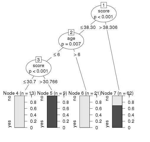
Conclusion
From the decision tree shown above we can conclude that anyone whose readingSkills score is less than 38.3 and age is more than 6 is not a native Speaker.
-
Integration and Interoperability
- R and Other Languages: R has increasingly integrated with other programming languages and tools. Packages like
reticulateallow users to run Python code within R, facilitating cross-language workflows. - Data Science and Machine Learning: R has become a go-to tool for data scientists. Its packages for machine learning (like
caret,mlr, andtidymodels) and its capabilities in data wrangling have made it indispensable in the field.
- R and Other Languages: R has increasingly integrated with other programming languages and tools. Packages like