Ingredients
Original recipe (1X) yields 4 servings
- 4 skinless, boneless chicken breast halves
- cayenne pepper to taste
- salt and ground black pepper to taste
- all-purpose flour for dredging
- 2 tablespoons olive oil
- 1 tablespoon capers, drained
- ½ cup white wine
- ¼ cup fresh lemon juice
- ¼ cup water
- 3 tablespoons cold unsalted butter, cut in ¼-inch slices
- 2 tablespoons chopped fresh Italian parsley
Directions
- Place chicken breasts between 2 sheets of heavy plastic on a solid, level surface. Firmly pound chicken breasts with the smooth side of a meat mallet to a 1/2-inch thickness.
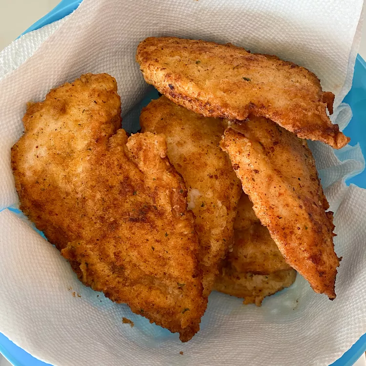
- Season both sides of chicken breasts with cayenne, salt, and black pepper; dredge lightly in flour and shake off any excess.
:max_bytes(150000):strip_icc():format(webp)/220751-QuickChickenPiccata-ddmfs-Step1-0534-27834128023e413093119fdfbc990319.jpg) Dotdash Meredith Food Studios
Dotdash Meredith Food Studios - Heat olive oil in a skillet over medium-high heat. Place chicken in the pan, reduce heat to medium, and cook until browned and cooked through, about 5 minutes per side; transfer to a plate.
:max_bytes(150000):strip_icc():format(webp)/220751-QuickChickenPiccata-ddmfs-Step2-0535-028e472b00f34d8c8c53bf8d1dc648f9.jpg) Dotdash Meredith Food Studios
Dotdash Meredith Food Studios - Cook capers in reserved oil, smashing them lightly to release brine, until warmed through, about 30 seconds. Pour white wine into the skillet and bring to a boil while scraping the browned bits of food off the bottom of the pan with a wooden spoon. Cook until reduced by half, about 2 minutes.
:max_bytes(150000):strip_icc():format(webp)/220751-QuickChickenPiccata-ddmfs-Step3-0536-e434e35233fa43c4a5c27e2aee6a7851.jpg) Dotdash Meredith Food Studios
Dotdash Meredith Food Studios - Stir lemon juice, water, and butter into the reduced wine mixture; cook and stir continuously to form a thick sauce, about 2 minutes. Reduce heat to low and stir parsley through the sauce.
:max_bytes(150000):strip_icc():format(webp)/220751-QuickChickenPiccata-ddmfs-Step4-0537-bbfce751600d40f1994c2faf1c6a8868.jpg) Dotdash Meredith Food Studios
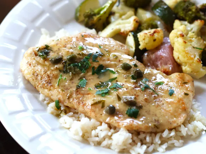
Dotdash Meredith Food Studios - Return chicken breasts to the pan and cook until heated through, 1 to 2 minutes. Serve with sauce spooned over the top.
:max_bytes(150000):strip_icc():format(webp)/222002-Chef-Johns-Stuffed-Peppers-DDMFS-3115-4x3-Ingredients-14575df7114f48d79e48b3a2de018534.jpg) Dotdash Meredith Food Studios
Dotdash Meredith Food Studios:max_bytes(150000):strip_icc():format(webp)/222002-Chef-Johns-Stuffed-Peppers-DDMFS-3117-4x3-Step-02-2e3bac6853f44aec83036fa833498984.jpg) Dotdash Meredith Food Studios
Dotdash Meredith Food Studios:max_bytes(150000):strip_icc():format(webp)/222002-Chef-Johns-Stuffed-Peppers-DDMFS-3121-4x3-Step-03-1c3e99153b56488fa35c2b48aa18973a.jpg) Dotdash Meredith Food Studios
Dotdash Meredith Food Studios:max_bytes(150000):strip_icc():format(webp)/222002-Chef-Johns-Stuffed-Peppers-DDMFS-3129-Step-04-b9e2574cce8d4eb3ad9cdd8fe07ba037.jpg) Dotdash Meredith Food Studios
Dotdash Meredith Food Studios:max_bytes(150000):strip_icc():format(webp)/222002-Chef-Johns-Stuffed-Peppers-DDMFS-3130-Step-05-e4f86bd2328849359c3894ec0834a9aa.jpg) Dotdash Meredith Food Studios
Dotdash Meredith Food Studios:max_bytes(150000):strip_icc():format(webp)/222002-Chef-Johns-Stuffed-Peppers-DDMFS-3171-Step-07-760304fc18874bfd8c29cfcf1eb50329.jpg) Dotdash Meredith Food Studios
Dotdash Meredith Food Studios:max_bytes(150000):strip_icc():format(webp)/222002-Chef-Johns-Stuffed-Peppers-DDMFS-3172-4x3-Step-08-a5509e34f0894ad88fbac054681efa2e.jpg) Dotdash Meredith Food Studios
Dotdash Meredith Food Studios
:max_bytes(150000):strip_icc():format(webp)/AR-236359-beef-and-rice-stuffed-bell-peppers-DDMFS-4x3-step-01-52e8ee2fe6aa46e580e8d589ccae79fe.jpg) Dotdash Meredith Food Studios
Dotdash Meredith Food Studios:max_bytes(150000):strip_icc():format(webp)/AR-236359-beef-and-rice-stuffed-bell-peppers-DDMFS-4x3-step-02-0fd0cbf56b5b4d8bbcff3acd99c1f008.jpg) Dotdash Meredith Food Studios
Dotdash Meredith Food Studios:max_bytes(150000):strip_icc():format(webp)/AR-236359-beef-and-rice-stuffed-bell-peppers-DDMFS-4x3-step-03-1eb1047747ef46b886d0e0222f49b016.jpg) Dotdash Meredith Food Studios
Dotdash Meredith Food Studios:max_bytes(150000):strip_icc():format(webp)/AR-236359-beef-and-rice-stuffed-bell-peppers-DDMFS-4x3-step-04-0ab049bb3dc7495db4f5cb92a89601d0.jpg) Dotdash Meredith Food Studios
Dotdash Meredith Food Studios:max_bytes(150000):strip_icc():format(webp)/AR-236359-beef-and-rice-stuffed-bell-peppers-DDMFS-4x3-step-05-72a5278305904adf8768700e19e11a98.jpg) Dotdash Meredith Food Studios
Dotdash Meredith Food Studios:max_bytes(150000):strip_icc():format(webp)/AR-236359-beef-and-rice-stuffed-bell-peppers-DDMFS-4x3-step-06-679640c9e6754b3a8ba21929c229c0d9.jpg) Dotdash Meredith Food Studios
Dotdash Meredith Food Studios:max_bytes(150000):strip_icc():format(webp)/AR-236359-beef-and-rice-stuffed-bell-peppers-DDMFS-4x3-step-07-5c20d6e8317a42f8b42ca06d6354f4e9.jpg) Dotdash Meredith Food Studios
Dotdash Meredith Food Studios
:max_bytes(150000):strip_icc():format(webp)/45957-ChickenMakhaniIndianButterChicken-mfs-Step1-0016-028c1e94e23d4387aff0b606dfee0b52.jpg) Dotdash Meredith Food Studios
Dotdash Meredith Food Studios:max_bytes(150000):strip_icc():format(webp)/45957-ChickenMakhaniIndianButterChicken-mfs-Step2-0017-48e3218ab32a46be85d3a8ad4a347233.jpg)
:max_bytes(150000):strip_icc():format(webp)/45957-ChickenMakhaniIndianButterChicken-mfs-Step3-0025-c994e98183444a8fb52860632cf9c1cb.jpg) Dotdash Meredith Food Studios
Dotdash Meredith Food Studios:max_bytes(150000):strip_icc():format(webp)/45957-ChickenMakhaniIndianButterChicken-Step4-0022-67d91823c76d40219d03ae51bc3ac576.jpg)
:max_bytes(150000):strip_icc():format(webp)/45957-ChickenMakhaniIndianButterChicken-mfs-Step6-0030-194934e58e6b4815b80034ab94bccde0.jpg) Dotdash Meredith Food Studios
Dotdash Meredith Food Studios:max_bytes(150000):strip_icc():format(webp)/45957-ChickenMakhaniIndianButterChicken-mfs-Step5-0026-24149cafdae948c4acf5ae7c0441b9b5.jpg) Dotdash Meredith Food Studios
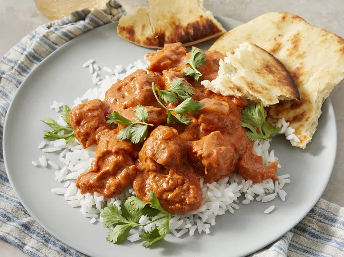
Dotdash Meredith Food Studios:max_bytes(150000):strip_icc():format(webp)/45957-ChickenMakhaniIndianButterChicken-mfs-4X3-0037-7aa9a555bf3943baae20c5c3b0921375.jpg)