Ingredients
1/2x1x2x
Original recipe (1X) yields 10 servings
- 3 cooked chicken breasts, diced
- 1 (2 ounce) bottle hot sauce
- 2 tablespoons butter, melted
- 1 (8 ounce) bottle blue cheese salad dressing
- 1 (16 inch) prepared pizza crust
- 1 (8 ounce) package shredded mozzarella cheese
Directions
- Gather the ingredients.
:max_bytes(150000):strip_icc():format(webp)/23735-buffalo-style-chicken-pizza-DDMFS-121-4x3-step-01-e1f3b42b561b42f7976f5c97cd3f68a1.jpg) Dotdash Meredith Food Studios
Dotdash Meredith Food Studios - Preheat the oven to 425 degrees F (220 degrees C).
- Mix chicken, hot sauce, and melted butter in a bowl until well combined.
:max_bytes(150000):strip_icc():format(webp)/23735-buffalo-style-chicken-pizza-DDMFS-122-4x3-step-02-f5946815dd39432a9b6c1e9eebcacfd3.jpg) Dotdash Meredith Food Studios
Dotdash Meredith Food Studios - Place crust onto a rimmed baking sheet or pizza pan. Spread salad dressing over crust.
:max_bytes(150000):strip_icc():format(webp)/23735-buffalo-style-chicken-pizza-DDMFS-129-4x3-step-04-8f39520c045b43eea4f7988b5c93a1bc.jpg) Dotdash Meredith Food Studios
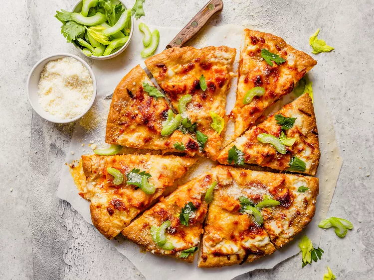
Dotdash Meredith Food Studios - Top with chicken mixture and sprinkle with mozzarella.
:max_bytes(150000):strip_icc():format(webp)/23735-buffalo-style-chicken-pizza-DDMFS-133-4x3-step-05-fa68f6230b9c40ada4c04059c44bac36.jpg) Dotdash Meredith Food Studios
Dotdash Meredith Food Studios - Bake in the preheated oven until crust is golden brown and cheese is bubbly, about 5 to 10 minutes. Let sit a few minutes before slicing.
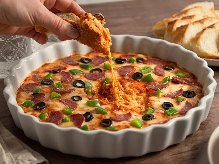
:max_bytes(150000):strip_icc():format(webp)/ALR-14803-hot-pizza-dip-VAT-step-01-0166266c45ce4a29aa4e202fc2a6e5a0.jpg) Allrecipes / Sonia Bozzo
Allrecipes / Sonia Bozzo:max_bytes(150000):strip_icc():format(webp)/ALR-14803-hot-pizza-dip-VAT-step-02-1-d07568e4d5d54be5b7066ae24dfd659a.jpg) Allrecipes / Sonia Bozzo
Allrecipes / Sonia Bozzo:max_bytes(150000):strip_icc():format(webp)/ALR-14803-hot-pizza-dip-VAT-step-03-f53aafa40b124f9583bf65edb7133da4.jpg) Allrecipes / Sonia Bozzo
Allrecipes / Sonia Bozzo:max_bytes(150000):strip_icc():format(webp)/ALR-14803-hot-pizza-dip-VAT-step-04-8bd18e35c31f4edcb6b97cbac492d668.jpg) Allrecipes / Sonia Bozzo
Allrecipes / Sonia Bozzo:max_bytes(150000):strip_icc():format(webp)/ALR-14803-hot-pizza-dip-VAT-step-05-bc6753efdb434303a94480f4d629b2ef.jpg) Allrecipes / Sonia Bozzo
Allrecipes / Sonia Bozzo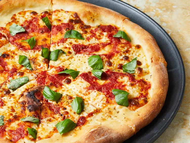
:max_bytes(150000):strip_icc():format(webp)/70801_BrickOvenPizzaBrooklynStyle_ddmfs_Shot1_3x4_3794-bfdc38cb60984cb69d930638acaee72a.jpg) Dotdash Meredith Food Studios
Dotdash Meredith Food Studios:max_bytes(150000):strip_icc():format(webp)/70801_BrickOvenPizzaBrooklynStyle_ddmfs_Shot2_3x4_3796-d13ee6986b7f4af5af2738fb2d10c157.jpg) Dotdash Meredith Food Studios
Dotdash Meredith Food Studios:max_bytes(150000):strip_icc():format(webp)/70801_BrickOvenPizzaBrooklynStyle_ddmfs_Shot2_3x4_3800-ecf5300d9b044bb6adfef191ce23917f.jpg) Dotdash Meredith Food Studios
Dotdash Meredith Food Studios:max_bytes(150000):strip_icc():format(webp)/70801_BrickOvenPizzaBrooklynStyle_ddmfs_Shot3_3x4_3805-208572f676254037a97b81ff46a33d3f.jpg) Dotdash Meredith Food Studios
Dotdash Meredith Food Studios:max_bytes(150000):strip_icc():format(webp)/70801_BrickOvenPizzaBrooklynStyle_ddmfs_Shot4_3x4_3842-92e01876be4f419e878154aa862dd459.jpg) Dotdash Meredith Food Studios
Dotdash Meredith Food Studios:max_bytes(150000):strip_icc():format(webp)/70801_BrickOvenPizzaBrooklynStyle_ddmfs_Shot5_3x4_3844-dfa3954cae6c4b75868c0a7a6e131579.jpg) Dotdash Meredith Food Studios
Dotdash Meredith Food Studios:max_bytes(150000):strip_icc():format(webp)/70801_BrickOvenPizzaBrooklynStyle_ddmfs_Shot6_3x4_3847-0dee41cde0d84db788493a58a95afc88.jpg) Dotdash Meredith Food Studios
Dotdash Meredith Food Studios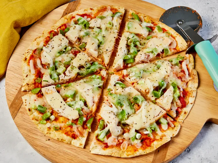
:max_bytes(150000):strip_icc():format(webp)/258013-easy-tortilla-pizza-DDMFS-097-step-01-94eaf97e4e6e4d64b499c5d557361fde.jpg) Photographer: Jen Causey / Food Styling: Jennifer Wendorf / Prop Styling: Julia Bayless
Photographer: Jen Causey / Food Styling: Jennifer Wendorf / Prop Styling: Julia Bayless:max_bytes(150000):strip_icc():format(webp)/258013-easy-tortilla-pizza-DDMFS-098-step-02-871442b02e08485cb87cf0f3a408a8df.jpg) Photographer: Jen Causey / Food Styling: Jennifer Wendorf / Prop Styling: Julia Bayless
Photographer: Jen Causey / Food Styling: Jennifer Wendorf / Prop Styling: Julia Bayless:max_bytes(150000):strip_icc():format(webp)/258013-easy-tortilla-pizza-DDMFS-099-step-03-b7b20d4148c04d858f31688500544683.jpg) Photographer: Jen Causey / Food Styling: Jennifer Wendorf / Prop Styling: Julia Bayless
Photographer: Jen Causey / Food Styling: Jennifer Wendorf / Prop Styling: Julia Bayless:max_bytes(150000):strip_icc():format(webp)/258013-easy-tortilla-pizza-DDMFS-100-step-04-8153762203634c43bfec5294f3426a65.jpg) Photographer: Jen Causey / Food Styling: Jennifer Wendorf / Prop Styling: Julia Bayless
Photographer: Jen Causey / Food Styling: Jennifer Wendorf / Prop Styling: Julia Bayless:max_bytes(150000):strip_icc():format(webp)/258013-easy-tortilla-pizza-DDMFS-103-step-05-715b88dc63254ea6a8a80847077e78b3.jpg) Photographer: Jen Causey / Food Styling: Jennifer Wendorf / Prop Styling: Julia Bayless
Photographer: Jen Causey / Food Styling: Jennifer Wendorf / Prop Styling: Julia Bayless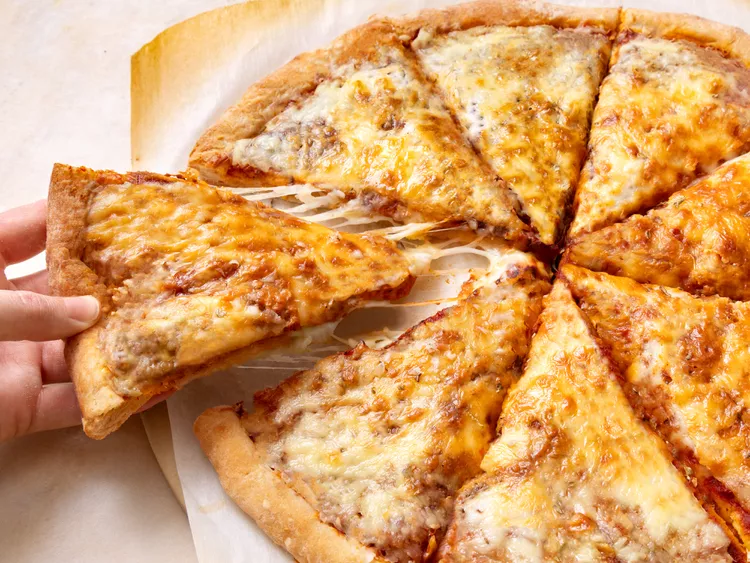
:max_bytes(150000):strip_icc():format(webp)/20171-quick-and-easy-pizza-crust-DDMFS-Step-1-cf69484242dd471bad8423280e7c7c65.jpg)
:max_bytes(150000):strip_icc():format(webp)/20171-quick-and-easy-pizza-crust-step2-215-4x3-f6ccf044c65647038caf0ee7e1c78664.jpg) Dotdash Meredith Food Studios
Dotdash Meredith Food Studios:max_bytes(150000):strip_icc():format(webp)/20171-quick-and-easy-pizza-crust-step3-216-4x3-870ed5d74fa74bdc86736041a9e5b439.jpg) Dotdash Meredith Food Studios
Dotdash Meredith Food Studios:max_bytes(150000):strip_icc():format(webp)/20171-quick-and-easy-pizza-crust-step4-220-4x3-9f6f2fe236754e2e8cc3779fc0f8ad9f.jpg)
:max_bytes(150000):strip_icc():format(webp)/20171-quick-and-easy-pizza-crust-step6-226-4x3-14feb9228539410b8a8eb9ab18fa6288.jpg) Dotdash Meredith Food Studios
Dotdash Meredith Food Studios:max_bytes(150000):strip_icc():format(webp)/20171-quick-and-easy-pizza-crust-step7-228-4x3-31bf7c6ba38b46b2af7dba80cc6730fa.jpg) Dotdash Meredith Food Studios
Dotdash Meredith Food Studios:max_bytes(150000):strip_icc():format(webp)/20171-quick-and-easy-pizza-crust-step8-229-4x3-ae83adff9a5c473789941a09b5a88978.jpg) Dotdash Meredith Food Studios
Dotdash Meredith Food Studios:max_bytes(150000):strip_icc():format(webp)/ALR-20171-quick-and-easy-pizza-crust-VAT-4x3-2-229693959a224d749b062d4eb8983351.jpg)
:max_bytes(150000):strip_icc():format(webp)/14522-Pizza-On-The-Grill084-step1-e860fd63c5fc4b2e8730386d3c1a197b.jpg)
:max_bytes(150000):strip_icc():format(webp)/14522-Pizza-On-The-Grill085-step2-251baa077a9f4f239aae5f380b778a94.jpg)
:max_bytes(150000):strip_icc():format(webp)/14522-Pizza-On-The-Grill086-step3-9b0c2e734c3247b097cd3973bd25eb2e.jpg)
:max_bytes(150000):strip_icc():format(webp)/14522-Pizza-On-The-Grill087-step4-764959af4c1e44b5998bcb56e7441ac0.jpg)
:max_bytes(150000):strip_icc():format(webp)/14522-Pizza-On-The-Grill088-step5-67e5ec8aa52245f0a271a6672e89c909.jpg)
:max_bytes(150000):strip_icc():format(webp)/14522-Pizza-On-The-Grill091-step8-4c2657cc05b040aaa399cbb2c532cd96.jpg)
:max_bytes(150000):strip_icc():format(webp)/14522-Pizza-On-The-Grill089-step6-c8129d968bcb44b38a1e232e7ad9a49d.jpg)
:max_bytes(150000):strip_icc():format(webp)/14522-Pizza-On-The-Grill092-step9-40fea257ae1f43f99d4556db7bb5f32f.jpg)
:max_bytes(150000):strip_icc():format(webp)/14522-Pizza-On-The-Grill093-step10-6aec17ffdbd246fb8d7dcf283d4c3bbb.jpg)
:max_bytes(150000):strip_icc():format(webp)/14522-Pizza-On-The-Grill094-step11-494736f8c5274578b4a17444e52ec24e.jpg)
:max_bytes(150000):strip_icc():format(webp)/14522-Pizza-On-The-Grill095-step12-a69d3d4051ba4f31876e9a68db2a795b.jpg)
:max_bytes(150000):strip_icc():format(webp)/14522-Pizza-On-The-Grill096-step13-368c7b7773e7417e82cfab673cbe1915.jpg) Dotdash Meredith Food Studios
Dotdash Meredith Food Studios
:max_bytes(150000):strip_icc():format(webp)/8887-Chicken-Marsala-mfs-STEPS-001-9fee3a782119400683e56bb8c64d234a.jpg)
:max_bytes(150000):strip_icc():format(webp)/8887-Chicken-Marsala-mfs-STEPS-006-5187238a4f2949eaa493ac5e0db5808b.jpg)
:max_bytes(150000):strip_icc():format(webp)/8887-Chicken-Marsala-mfs-STEPS-009-8e94c96e9db54197b7d94649d949e8d3.jpg)
:max_bytes(150000):strip_icc():format(webp)/8887-Chicken-Marsala-mfs-STEPS-011-a07c93c3ed1b4eaeb3fc10c8075035be.jpg)
:max_bytes(150000):strip_icc():format(webp)/8887-Chicken-Marsala-mfs-STEPS-015-6b4a33fe296b4d12815216da9a5e879b.jpg)
:max_bytes(150000):strip_icc():format(webp)/8887-Chicken-Marsala-mfs-STEPS-017-8036ec13133b4e8783151dd51116385f.jpg)
:max_bytes(150000):strip_icc():format(webp)/62696-chicken-parmesan-casserole-VAT-001-step-01-7c1a00b6a0524ea7a0fdd4ca503b4b4a.jpg)
:max_bytes(150000):strip_icc():format(webp)/62696-chicken-parmesan-casserole-VAT-002-step-02-4ab38d8286d8434b812c7068d910e677.jpg)
:max_bytes(150000):strip_icc():format(webp)/62696-chicken-parmesan-casserole-VAT-003-step-03-5696d423f5004a80b71c78224b448da7.jpg)
:max_bytes(150000):strip_icc():format(webp)/62696-chicken-parmesan-casserole-VAT-005-step-04-5acd75c8002c4e68908b5e62c1dba03c.jpg) Allrecipes / Sonia Bozzo
Allrecipes / Sonia Bozzo:max_bytes(150000):strip_icc():format(webp)/62696-chicken-parmesan-casserole-VAT-006-step-06-6ea9de2901fd46c7a71ca5e58057f4eb.jpg)